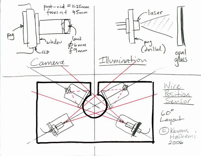
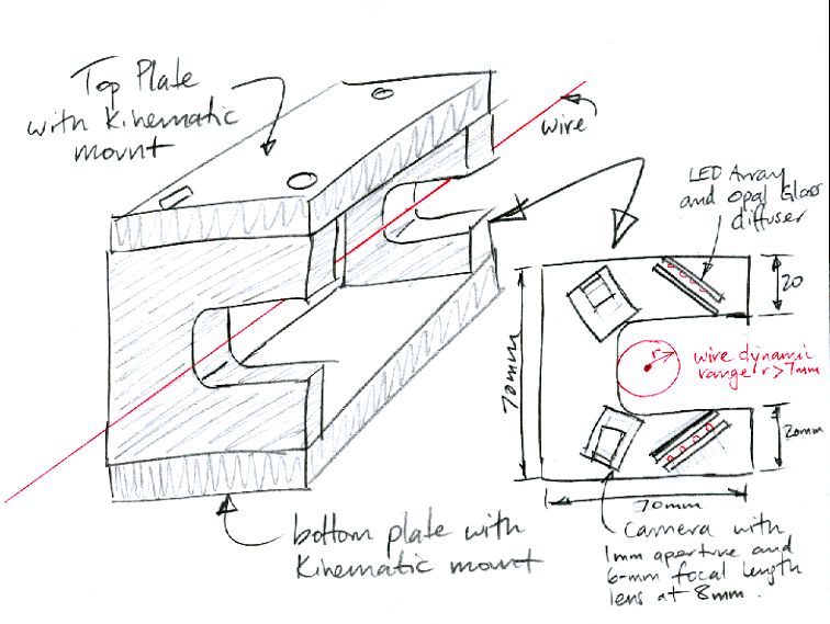
Figure: Preliminary Sketch. Shows the two cameras and accompanying sources of illumination.
At CERN in November 2006, we visited a test stand of Helene Durand's that consisted of stretched wires over 100 m long, each being monitored by wire position monitors (WPSs). Each wire had five or six WPSs along its length. The stretched wire provides a reference line with which to align components such as accelerator magnets and beam pipes. The wire is straight in the horizontal direction, but sags in the vertical direction. Helene proposes to determine shape of the wire sag by a combination of calculation and calibration.
The existing WPSs at CERN are model WPS2-D sensors made by Fogale Nanotech. We could not find their sensor data sheet on their website, but you can get a version in French from us here. The WPS2-D data sheet claims a resolution of 0.3 μm in measurement of wire position across a 10-mm dynamic range in the vertical and horizontal directions. But the linearity of the instrument is only 0.15 mm. There is coupling between the vertical and horizontal measurements, so that a 10-mm movement vertically gives an apparent 0.8-mm movement horizontally. The main disadvantage of the sensor, however, is its cost. According to Helene, these sensors cost $5000 in quantity ten, and $3000 in quantity one thousand.
We proposed that OSI design and develop an optical WPS that will provide 2-μm resolution and 5-μm absolute accuracy across a 10 mm × 10 mm dynamic range, and which will cost $2000 in quantity or less in quantity ten, and $500 in quantity one thousand. Helene expressed interest in our proposed sensor, and we began development immediately upon our return from Europe.
In the sections below, you will see our development described as it proceeds. Please note that all our work is protected by the GNU Public License.
Our proposed WPS (Wire Position Sensor) consists of two cameras looking at a wire from two different directions. As the wire moves up and down, or side to side, the cameras take pictures, and image analysis determines the position of the wire image upon each image sensor. A calibration procedure performed by Open Source Instruments supplies us with the geometric parameters we need to translate the wire image position into the position of the wire with respect to the kinematic mount of the entire sensor structure.
Illumination for the wire images comes from red laser light shining upon opal glass diffusers. The wire image is a black line on a white background. Because the wire extends across the height of the image, we can obtain a crude measurement of the orientation of the wire within the sensor cavity as well.
The WPS provides a slot through which you can lower the wire, and therefore place the sensor along the length of a stretched wire without taking the sensor apart or re-stringing the wire through the sensor aperture. To allow for this slot, the cameras look at the wire from two different directions at 120 degrees to one another, instead of the optimal 90 degrees.
The WPS measurement is stable to the extent that the position of the image sensor and its lens is stable with respect to the kinematic mounting block.
Although there is no outward similarity between the two instruments, the WPS is very similar to another optical instrument called the BCAM. The BCAM locates white spots of light on its image sensor, and so monitors the movements of light sources to 5 μrad across its 30 × 40 mrad field of view. The WPS locates dark stripes on its image sensor, and so monitors the movements of wires to 40 μrad across its 200 × 300 mrad field of view. The wire is 45 mm from the cameras in the above prototype design, so the WPS will be accurate to 2 μm within its dynamic range of ±5 mm.
By rotating the WPS in a known way about a fixed wire, we will be able to calibrate the WPS so that it gives us the absolute position of the wire with respect to the WPS kinematic mount, with accuracy better than 5 μm.
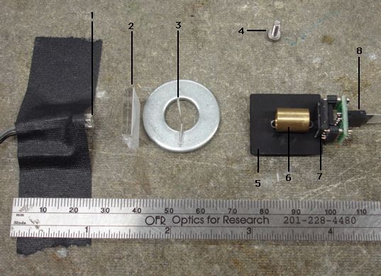
With the help of super-glue and a few parts we had lying around in the lab, we made the WPS camera breadboard shown below. We had to put a cardboard box over the entire camera when we took photographs, in order to block ambient light.
Our original plan was to use a red laser diode as our source of illumination. But we quickly found that the laser light, even after passing through the diffuser, showed bright points of light and sharp points of darkness. These features are known as laser speckle, and they arise with coherent, monochromatic light. We exchanged the laser for a bright red LED (light-emitting diode).
The lens holder provides a 3-mm aperture and holds a 6-mm diameter 9-mm focal length plano-convex lens (Edmund Optics part 32469). The focal point of the lens is roughly 14 mm from the image sensor. At 30 mm from the lens we took the following picture of an M2.5 screw.
The screw pitch in the image is 21 pixels. Each pixel is 10 μm, and the actual pitch of the screw is 0.45 mm. The image magnification is 0.47. We expect it to be 14 mm / 30 mm = 0.47. The diameter of the thread is 2.5 mm on the screw and 107 pixels on the image. The image sensor itself is 320 pixels across, to the camera's field of view is roughly 7.5 mm at a range of 30 mm. With our magnification of 0.47, and the image sensor 3.2 mm across, we expect a field of view of 6.8 mm. When we moved the screw towards and away from the camera, we could discern individual threads from ranges 25 mm to 35 mm.
We now took a photograph of a wire. We clipped the wire off a through-hole capacitor, bent it with pliers, and glued it to a washer you see in the photograph above. In the camera, the wire appears as you see below. The wire diameter is 23 pixels in the image at a range of 30 mm. Our measured magnification of 0.47 implies a wire diameter is 0.5 mm.

At first we tried to determine the position of the wire in the image by negating the image intensity and finding the intensity centroid of the wire using our BCAM instrument analysis. But that did not work well. The light intensity in the wire image varies from bottom to top, and shifts the centroid. You can see this as an upward shift of the red cross in the image below.
We had better success dividing the negated wire image into vertical segments, and taking the centroid of each segment. Even within a segment, however, we noticed the centroid moving from left to right because the intensity across the wire was not uniform. In practice, we can expect ambient reflections off the wire. Even if these are not as bright as the diffuse background, they will displace the apparent center of the wire.
When we look at the differentiated image of the wire, which we call the gradient image, we find that the wire edge is defined sharply, and is insensitive to variations in the background illumination and to reflections off the wire.
Our Rasnik Instrument analysis uses horizontal and vertical gradient images to find the edges of rows and columns of chess-board squares. With a sharp image, the analysis locates a rasnik pattern with resolution 1 μm on the image sensor. With our magnification of 0.47, this 1 μm would translate to 2 μm in wire position. We are confident that we can fit two straight lines to the edges of the wire as they appear in the gradient image, and so obtain the location of the center of the wire to 2 μm resolution, its orientation with resolution 500 μrad, and its range from the camera with resolution 100 μm.
Suppose we have a wire stretched along the top of a granite table. We would like to place our WPS around the wire at any point without disturbing the wire. We would like to be able to do this quickly, without having to unscrew a cover and screw it back on again. We would like to be able to rotate the WPS so we can check that its measurements are self-consistent.
After thinking about these constraints for a while, we arrived at the following design for the enclosure.
This enclosure will mount either on its top plate or its bottom plate. Both have a cone, slot, flat kinematic mount like the ones on the underside of BCAMs. The cone balls of the two mounts are on the same side as the cameras.
As you can see, the cameras now face up and down. They are now more sensitive to movement in the horizontal direction than to movement in the vertical direction. Instead of a single LED shining on a diffuser, we use an array of LEDs. This means we can, at the same time, make the diffuser larger and move the LEDs closer to it. We switch to a 6-mm lens so we can reduce the distance between the camera and the wire. The shorter focal length means a shorter distance between the lens and the image sensor, and therefore a wider field of view. To reduce the camera's sensitivity to ambient light, we decrease its aperture diameter to 1 mm or even 500 μm. The smaller aperture will also increase the camera's depth of field.
This enclosure allows us to calibrate the WPS as follows. With a CMM (computer measuring machine), we mount the WPS on three balls, and measure the front corner of its mounting plate, and the direction of one of its long sides. This defines a coordinate system on the WPS chassis. We rotate the WPS and mount it upside down on the same three balls, and measure the same parts of the plate. This gives us the new location and orientation of the same coordinate system. Now we know how the WPS moves when we rotate it.
We place the WPS around a wire and take images from its camera. We rotate it and do the same thing again. Our wire, meanwhile, is mounted upon a micrometer stage. We move the wire 5 mm to the left and measure with both orientations. We move it 5 mm up, and so on. With wire positions and two orientations of the sensor, we obtain a robust, absolute calibration of the device, even though we don't at first know where the wire is with respect to the mounting balls. With this procedure, we never have to measure a wire directly. The trick of rotating the sensor gives us the wire position and the sensor calibration by the time we are done.
The wires used with the Fogale WPS are made of carbon fiber. Carbon fiber wires are strong and light, and so sag less than metal wires. The table below compares the properties of metals and carbon fiber, and shows that the ratio of strength to weight for carbon fiber is over a factor of ten higher than that of metals.
| Material | Density (g/cm3) | Strength (GPa) | Modulus (GPa) | 100-m Sag (mm) | CTE ppm/K |
|---|---|---|---|---|---|
| Carbon Fiber | 1.8 | 3 | 300 | 7.5 | -0.5 Longitudinal |
| Aluminum | 2.7 | 0.5 | 70 | 68 | 25 |
| Tungsten | 19.3 | 1.5 | 400 | 160 | 4 |
| Steel | 7.5 | 1 | 200 | 94 | 17 |
| Copper | 8.9 | 0.2 | 120 | 560 | 17 |
| Vectran® | 1.1 | 2.7 | 70 | 5.1 | <20 |
| Dyneema® | 0.98 | 3.4 | 110 | 3.6 | <20 |
Carbon fiber contracts with temperature in the direction of the fibers (the longitudinal direction), while the fibers themselves get thicker (in the lateral direction).
A hanging wire takes the shape of a catenary. If we are to calculate the vertical sag of a wire along its length to a few microns, we shall have to use the catenary equation in our calculation. But for now, we would like merely to estimate the sag of a 100-m wire, so we'll assume the wire describes a parabola as shown below.
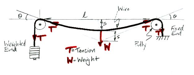
Whatever the shape of the wire, we see that 2Tsinθ = W, or sinθ = W/2T. The weight of the wire is lAρg, where g is gravity, ρ is the wire density and A is its cross-sectional area. We assume θ is small, so θ ≈ sinθ = lAρg/2T. The sag of the wire, in our parabolic approximation, is lθ/4. The minimum sag occurs with maximum tension in the wire. The maximum tension we can apply to a wire is, MA, where M is the wire material tensile strength. The minimum sag for length l is therefore smin ≈ l2ρg/8M. We note that the sag depends upon the ratio of density to strength, and is independent of the diameter of the wire.
For a carbon-fiber wire 100 m long, we expect a sag of 7.5 mm when the wire is stressed to its breaking strength of 3 GPa. If we use tungston wire, the sag would be 160 mm. Clearly, we should try to use carbon fiber wires, as recommended by Fogale, and as we saw in use at CERN. Helene tells us that her wires at CERN have the following properties. Their wires are stretched by weights of 15 kg to a stress of 1 GPa. This gives them a sag of 20 mm over a 100-m stretch.
| Property | Value | Unit |
|---|---|---|
| Diameter | 400 | μm |
| Mass per Unit Length | 235 | g/km |
| Coefficient of Thermal Expansion | −1 | ppm/°C |
| Young's Modulus | 294 | GPa |
| Strength | >1 | GPa |
Carbon fiber wires tend to fray. Individual fibers separate from the wire, and the wire starts to untangle. To constrain these fibers, the wire manufacturer wraps the wire with two thin plastic threads that wind in opposite directions. Click here for a close-up photograph of three such wires with different wrappers. We estimate that the wires in the photograph are 700 μm thick.
With two thin wrappers in opposite directions, we estimate that the effect of the wrapper upon both the capacitive WPS and our proposed optical WPS will be less than 3 μm.
[09-OCT-08] Carbon fiber is a poor conductor of electricity, but it does conduct, and its poor conduction is necessary for the operation of capacitive sensors. But carbon fiber wires are fragile. They depend for their integrity upon their plastic wrapper. The wrapper is easy to displace along the wire. The wire itself is strong, but it is brittle. It breaks easily when you crimp or clamp it. It creeps over time, resulting in fibers popping out of the braid. Loose fibers are visible in our optical system, and also affect the measurement of capacitive systems.
The optical wire position sensor prefers a uniform, black wire. It does not need the wire to conduct electricity. Polymer fibers can be dyed black, and some are exceptionally strong. They attain their strength by stretching far beyond the breaking strain of metals and carbon fiber. Vectran®, for example, which we include in the table above, stretches by almost 4% before it breaks. Carbon fiber stretches only 1% before it breaks, and tungsten only 0.4%.
Friedrich Lackner at CERN has obtained some vectron wire. We obtained our data for vectron fibers here. Vectron fiber strength is 27 g/denier. A one-denier fiber is a fiber 9 km long that weighs one gram. The density of vectron is 1.1 g/cm3, so a 1-denier fiber has diameter 10 μm and cross-section 10-10m2. The breaking stress is therefore 2.7 GPa, which compares well with the 3-GPa breaking strain of carbon fiber.
A braided Vectran® wire is non-conducting and strong. It is not suitable for capacitive wire position sensors, but it is well-suited for optical sensors. A 100-m Vectran® wire loaded to its breaking strain will sag only 5 mm, while a carbon fiber wire loaded to its breaking strain will sage 7.5 mm. Vectran® can be dyed various colors, including black, to minimize optical reflections. It does not creep, it needs no binding threads, its fibers do not poke out of the weave. It is tough and resists moisture and hot air.
Suppose we have a piece of equipment several hundred meters long and we want to use wires as a straight-line reference with which to align it. We cannot string a single wire along the entire length of our equipment. Instead, we can string overlapping lengths of wire. This works well in the horizontal direction, but in the vertical direction we have the sag of the wire to contend with in addition to the overlap.
Our WPS sensors will be calibrated absolutely with respect to their kinematic mounting balls. When we have three WPSs on the same plate, as shown in the figure above, we can measure the relative positions of all three wires by using the calibration constants of each WPSs and combining them with a CMM measurement of the mounting balls on the plate itself.
We can describe each wire as a catenary with seven free parameters: the three coordinates of each end and the sag in the middle. Our y-coordinate is vertical, and z is along the wire. We assume we know the z-position of each WPSs in our system to within 1 cm by independent means. When we know our position to 1 cm along a 100-m wire that sags by 20 mm, we can determine the sag of the wire to 2 μm. That leaves five remaining unknown parameters per wire: the x-y coordinates of each end, and its sag.
The overlapping wire system contains a sequence of reference stations like the one shown above. At each station, two wires come to an end with weights, and another wire presents the maximum sag at its center. The three WPSs at each reference station provide the x-y coordinates of each wire with respect to the mounting plate.
We assume we know the z-position of each reference station to within a centimeter, just as we know the z-position of each WPS. Let us assume for the moment that we can orient the reference station so that its own coordinates are parallel to our global coordinates. We might do this with the help of a precision level and an auto-collimator. If we assume that the the coordinates of the plate are parallel to our global coordinates, only the x- and y-position of the plate remain to be determined.
We make six measurements per plate. We have five free parameters per wire, and two free parameters per reference station. On average, we have one wire per reference station. So we have six measurements and seven unknowns. We cannot solve for the wire position with these measurements alone.
Suppose we add another station between each reference station. We can call these the pilot stations. Each pilot station monitors two wires. It creates four measurements, and presents two new unknowns. We now have one reference station and one pilot station per wire. We have ten measurements and nine unknowns. We can solve for the wire shape, and the locations of both stations.
Provided we can orient each station with sufficient accuracy, we see that with alternating reference and pilot stations, we do not need to measure the sag of the wires. Our measurements will determine the sag for us. We assume, of course, that the shape of each wire follows the shape of a catenary to within a few microns along its length.
But orienting the stations with sufficient accuracy is a challenge on its own. With the help of an Inclinometer (A2065) we could measure the orientation of the plate with respect to vertical to an accuracy of 500 μrad. The two wires that come to an end on a reference station are 10 cm apart in the z-direction. If we are uncertain of the direction of the station's z-axis, we will be uncertain of the relative y-position of the two wires. With 500 μrad uncertainty, we get 10 cm × 500 μrad = 50 μm uncertainty in y-position. With the help of a BCAM we could measure the orientation of consecutive plates with respect to the wire direction to 50 μrad. The single wire is 10 cm from the wire ends, so a 50-μrad uncertainty in z-direction gives us a 5-μm uncertainty in the relative x-position of the single wire.
If we want 5 μm accuracy along our overlapping system of wires spaced 10 cm apart, we must know the orientation of each plate to at least 50 μrad. Because large pieces of equipment deform on the level of 50 μrad, we would have to measure the three orientations of each plate continuously.
One solution to this problem is to make a larger WPS, with dynamic range -20 mm to +2 mm in the vertical direction, and -10 mm to +10 mm in the horizontal. Each reference station has a single WPS with three wires passing through it, and each pilot station has a single WPS with two wires passing through it. We arrange the wires as shown below.
Each WPS must have enough dynamic range to accommodate three wires at once, one of which may be sagging with respect to the others by 20 mm. Because the wires are separated by only 10 mm, we need know the orientation of the plate to only 500 μrad. This we can do easily with an Inclinometer (A2065) for rotation about z and x, and a BCAM for rotation about y.
The problem with running several wires through a single WPS is that they might obscure one another in the field of view of one or both of the WPS cameras. With some care, however, we can set up the wires so that they do not obscure one another, and still leave them ±1 mm of movement.
These thoughts make us hopeful that we can build a WPS system in which the sag of each wire is determined by the system itself, without any need for calibration with weights, nor any need for calibration of the station positions after intallation.