Feasability Test for Subcutaneous Transmitter: Downshifting Receiver
© 2004, Kevan Hashemi,
Open Source Instruments Inc.
Contents
Introduction
Noise and Interference
Received Power
Bit Transmission
Favorable Transmission Directions
Conclusion
Introduction
The Downshifting Receiver (A3001B) section of our Rat Transmitter Test Board (A3001) contains an antenna input amplifier (U1) with a minimum gain of 10 dB (that's a factor of three in voltage amplification). The input amplifier provides the RF (radio frequency) input to the frequency mixer (L1). We also have an oscillator made out of the same voltage-controlled oscillator chip (U5, MAX2624) we used in our Modulator-Transmitter. The Downshifting Receiver provides tuning (T) and shutdown (S) inputs to the VCO just as did the Modulator-Trasmitter. In the following experiments, we leave the S input open, to enable the VCO, and connect the T input to 0V with a 50-Ohm BNC terminator so as to set the VCO output frequency to around 900 MHz.
The output of the VCO is -3 dBm (150 mV rms across a 50-Ohm load). Our frequency mixer (L1) requires an LO (local oscillator) input of at least +7 dBm, so the Downshifting Receiver amplifies the output of the VCO by +10 dBm (U2) to obtain the required +7 dBm (that's 0.5 V across a 50-Ohm load) for the mixer.
The mixer (L1) is the part that performs the downshifting. Both the RF and LO inputs to the mixer are periodic, and nearly sinusoidal. The mixer multiplies the two signals together. It is a non-linear device made out of diodes and a couple of transformers. The one we use is the ADE-2ASK from Minicircuits. We won't take the time here to explain how it works. The Minicircuits web site provides some application notes that don't go so far as to tell you how mixers work, but do provide schematics of the various types. The ADE-2ASK is a double-balanced mixer.
The mixer, as we said, multiplies the RF and LO inputs, and when we say multiply we mean multiply in the most literal sense. The mixer takes sin(2.pi.f1.t), where f1 is the RF frequency and t is time, and multiplies it by sin(2.pi.f2.t), where f2 is the LO frequency, to produce at its IF (intermediate frequency) output the product sin(2.pi.f1.t).sin(2.pi.f2.t). Of course, there is also a little of the LO frequency thrown in at the IF output, but we will later eliminate the LO frequency with a 150 MHz low-pass filter. The LO frequency, you will recall, is 900 MHz.
As we are sure you recall from your early trigonometry lessons, the product of the sinusoids of two angles is equal to the sum of two sinusoids, one of the difference angle, and one of the sum angle. Thus the output of the mixer contains one sinusoidal waveform at frequency f1-f2, and another at f1+f2. Our 150 MHz low-pass filter will knock out the f1+f2 term, because it will be between 1.8 GHz and 1.9 GHz. After the low-pass filter (which we plug into P3) we will be left with only the f1-f2 term, which we call the Intermediate Frequency (IF). The IF signal amplitude is proportional to the RF input amplitude. An ideal mixer would give us an IF term half the amplitude of the RF input, which is a -6 dB power drop from RF to IF. According to our mixer's data sheet, its conversion loss is less than -8 dB (a factor of 2.5 voltage attenuition).
If the voltage at the base of the Receiver's antenna is 200 uV at 950 MHz (that's -60 dBm in RF power terms), the RF input to our mixer will be 600 uV, and the IF output will be roughly 300 uV. If the LO frequency is 900 MHz, then the IF frequency will be 50 MHz. When the antenna signal frequency changes to 1000 MHz, the IF frequency changes to 100 MHz. The mixer downshifts the antenna signal by 900 MHz (the LO frequency).
The Downshifting Receiver amplifies the IF by 10 dBm and delivers it to P3, a BNC plug (OUT in the schematic). The IF output frequency is equal to the antenna frequency minus the LO frequency of 900 MHz, and the IF output amplitude is equal to the antenna amplitude multiplied by four (+12 dBm). We can plug our 150 MHz coaxial low-pass filter into P3 if we like, and so look at only the IF signal, or we can leave off the 150 MHz filter and see also the LO signal that leaks through the mixer onto the IF output.
What we want to do with the Downshifting Receiver is determine whether or not we can receive a signal through space from the Modulator-Tranmsitter, from one antenna to another, whether that signal is large enough to make the Rat Transmitter idea possible, and whether we can transmit data bits at sufficient speed to keep our transmission bursts down to 5 us every 2.5 us (Transmitter).
Noise and Interference
It took us an hour or so to get the Downshifting Receiver working. We had chosen a higher-gain amplifier chip to play the part of U1 and U3 in the circuit (the ERA-3SM from Minicircuits), but these amplifiers proved to be unstable, generating their own RF noise. We replaced them with ERA-1SM (also from Minicircuits) and the noise vanished. We also found that we needed a few more decoupling capacitors on the supply lines to cut down on the LO content of the IF output.
With the Downshifting Receiver working, we added an antenna wire 100 mm long,
the same length as the antenna we arrived at in our experiments with the
Modulator-Transmitter. We turned on the Modulator-Trasmitter, and connected a 0V to 3 V triangle
wave to its tuning input (T). We know from our previous work that the frequency generated by the
VCO on the Modulator-Transmitter (U2) varies between rouglhy 900 MHz and 1000
MHz (1 GHz) as the tuning input varies from 0 V to 3 V.
We connect our oscilloscope to the IF output of the Downshifting Receiver, with a 150 MHz low-pass filter in the IF line to knock out higher frequencies. Our oscilloscope can see the IF output directly, with no loss in amplitude, because the IF is below 150 MHz, and our oscilloscope has bandwidth 300 MHz. Figure 1 shows the two circuits separated by 20 cm on our bench.
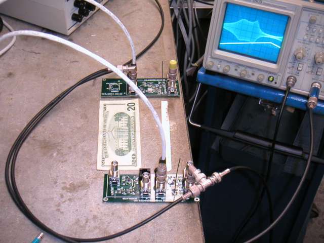
Figure 1: The Modulator-Transmitter (bottom) and Downshifting Receiver (top), their antennas separated by 20 cm, and the transmission performance displayed on the oscilloscope. Note the 75-mm green antenna wire sticking up from each circuit, and also the blue 150-MHz coaxial low-pass filter inserted in the IF line as it enters the oscilloscope.
The first thing we did, after rejoicing at the sight of received RF power, was to cut off the transmitter antenna. The IF signal decreased to less than 1 mV amplitude. We unplugged the transmitter from its power source, and the IF signal collapsed to white noise of amplitude less than 0.5 mV. We expect at least 0.5 mV of white noise on any oscilloscope input, so all we can deduce, from this 0.5 mV of noise, is that the noise internal to the receiver, and interference picked up in our lab by the receiver antenna, is not greater than 0.5 mV at the IF output, or roughly 100 uV and 300 pW at the base of the antenna.
Received Power
We restored the transmitter antenna and clipped it back until we saw the largest IF amplitude over the widest range of transmitter frequency. We found that the antenna was now 75 mm long, not the 100 mm we had arrived upon previously. In theory, this makes sense, because the wavelength of 1 GHz in air is 30 cm, so a quarter-wave antenna would be about 75 mm long.
What is good for the transmitting antenna should also be good for the receiving antenna, so we cut back the receiving antenna to 75 mm, and the received power jumped up again. Figure 2 shows the IF output from the receiver when the two circuits are separated by 20 cm. As you can see, the IF output reaches 30 mV at the upper end of the VCO frequency range, when the IF frequency is roughly 100 MHz.
Figure 2: IF output from the Downshifting Receiver (upper trace, 10 mV per division) and TUNE input to the Modulator-Transmitter (bottom trace, 0.5 V per division) with the two circuits separated by 20 cm. Note the peak in power reception at the upper end of the VCO frequency range.
We have 30 mV at the IF output, which means the antenna has roughly 8 mV, or 1 uW. We previously concluded that our transmitter was radiating roughly 300 uW into space. If our 75-mm antenna presents a 50 cm^2 aperture to the radiated power at a range of 20 cm, then we expect it to pick up 1% of this 300 uW, or 3 uW. We are seeing 1 uW at roughly 1 GHz, decreasing to 100 nW at around 920 MHz (if we assume the typical relationship between TUNE input and output frequency for our VCO).
We do not yet understand why our IF amplitude drops when the IF is less than 100 MHz, but when we changed the Downshifting Receiver's LO frequency to 950 MHz, we received 1 uW when the transmitter was running at 900 MHz. We conclude that our antenna and transmitter work fine from 900 MHz to 1 GHz, but we have an error in our Downshifting Receiver that is causing it to attenuate IF frequencies below 100 MHz. Perhaps we put a 100 pF capacitor in place of a 10 nF capacitor. We are confident that we can fix the problem in the long run.
At 1 GHz, we receive 30% of the power we expect when we assume that the receiving antenna presents an energy-absorbing aperture equal to the square of its length. We are not particularly confident in this assumption. Perhaps the effective aperture of our antenna is only 75 mm by 30 mm, in which case we are receiving 90% of the power we expect to receive. In any case, in logarithmic terms, our power transmission close to perfect.
Bit Transmission
We now modulate the transmitter frequency by driving the Modulator-Transmitter's T input with a square wave, and we observe the consequent modulation in the Downshifting Receiver's IF frequency and amplitude. It is not so easy to see changes in frequency on the scope, so we make use of the poor response of our receiver to 930 MHz transmissions, and modulated the transmitter frequency between 930 MHz and 1 GHz, to give us bursts of 100 MHz IF at the IF output (P3, called OUT in the schematic).
Figure 3: IF output from the Downshifting Receiver (upper trace, 5 mV per division) and TUNE input to the Modulator-Transmitter (bottom trace, 0.5 V per division) with the two circuits separated by 1 m. Note that the IF amplitude at 1 m range is 10 mV.
The oscilloscope trace shows clearly that the IF responds to the modulation of the transmitter frequency. We have clear transmission of logic levels at 10 MBPS (ten megabits per second), and we are confident that a properly-designed receiver could extract twenty megabits per second. We already know that the transmitter can modulate its output at twenty megabits per second.
Favorable Transmission Directions
No practical transmitter can radiate power uniformly in all directions. The only way we have to radiate electromagnetic waves is to move electrons back and forth, or around in circles. We cannot simply create charge and then annihilate it, which is what you have to do to get uniform power radiation in accordance with the inverse-square law of electric fields. Practical transmitters radiate power in some directions more than in others, depending upon the shape of the transmittig antenna. With our transmitter embedded in the body of a rat, we will find that the transmitting rotates as the rat moves around and rolls about, so we must be sure that we will receive enough power from the transmitter even when it is held in an unfavorable orientation with respect to our receiver.
We can easily deduce the relative power radiation in any direction by imagining that we are watching from the receiving antenna as electrons in the transmitter get pumped out of the transmitter ground plane and onto the antenna by the oscillator, and then pumped back again, in a continuous oscillation at 1 GHz. If we can see transverse motion of electrons from the receiver, then we will receive a strong signal from the transmitter. In the case of our straight wire antenna, we will receive a strong signal if the length of the antenna is perpendicular to our line of sight. If, on the other hand, we are looking down the length of a stright wire antenna, the electron movement is towards and away from us along the wire, and we will see very little transverse movement of electrons. When we are looking down the length of a straight wire antenna, we receive a weak signal.
Our receiver antenna is more sensitive to signals arriving from certain directions than in others, in exactly the same way as a transmitting antenna. If a straight wire antenna is perpendicular to direction of the incoming electromagnetic waves, we receive a strong signal. We are not as concerned about the receiver orientation, however, because we can keep the receiver stationary in the middle of the laboratory. A vertical wire antenna would receive signals from everything in the laboratory at or near the same height above the floor as itself. It is the transmitting antenna that we must worry about.
In theory, we might get no power at all from our transmitter when its antenna is pointing straight towards our receiver. But electromagnetic waves reflect off conducting surfaces, and scatter through near-conducting matter, so that even if the transmitter radiates its power away from the receiver, some of the power will arrive at the receiver by reflection. We can use this reflected power so long as the all reflected waves carry the same data bit. That is to say: when the transmitter is transmitting a 950 MHz signal to represent a logic zero, all reflected waves must be 950 MHz for a significant portion of the bit transmission time. In our case we plan to transmit at 20 MBPS, so our bit transmission time is 50 ns. A radio wave travels 15 meters through air in 50 ns, so our reflections will be useful so long as the difference in path lengths between the direct and various reflected waves is less than 15 m. If our receiver is only 3 m from the transmitter, then all the strongest signals arriving at the receiver will have path lengths within a couple of meters of one another, so we will be able to use the reflected waves.
We held our transmitter at range 1 m from the receiver and rotated it in all directions. We found that the received power varied by almost a factor of ten (10 dB). The IF output from the receiver varied from 10 mV down to 3 mV. We conclude that with a straight-wire antenna, we can use 10 dB as the potential power loss due to poor orientation of the transmitter.
At present, we plan to use a straight quarter-wave antenna inside the rat's body. Because of the high dielectric constant (80) of mammalian bodies, the length of this antenna will be far shorter than our present 75-mm antennas. The most efficient length might be as short as 10 mm. The transmitter circuit itself will be 18 mm square, so we do not expect the antenna to present any additional space problems.
Nevertheless, let us consider what would happen if we folded the transmitting antenna around so that it lay flat on the body of the transmitter. Instead of seeing electrons going back and forth, our receiver will see them going around in a loop. We will observe circulation of charge instead of displacement. Furthermore, we would see this circulation only from two particular directions, along the axis of the circulation. In other directions, we would see hardly any circulation, and no displacement either. This loop antenna might be worth trying, but we suspect that we will lose more than 10 dB in the unfavorable transmission directions.
Conclusion
Of the 300 uW we believe our Transmitter radiates into space, we receive 1 uW at range 20 cm, and 100 nW at range 1 m. We expect the power we receive to decrease in proportion to the square of the range, so at range 3 m we expect to receive 10 nW. We observe that the received power can vary by a factor of ten as we rotate the transmitter, so we can be sure of receiving 1 nW at range 3 m for all orientations of the transmitter.
We can purchase for around $100 a 1-m long antenna with effective aperture is ten times the area of the antenna we tested above. It will receive ten times as much power as the antenna we tested. With such an antenna, we will receive at least 10 nW at range 3 m from our transmitter.
Work done at Surrey University, England, suggests that we will lose up to 1 dB of power per cm through a rat's body, and almost 5 dB by reflection when passing from the rat's body (dielectric constant close to 80) into air (dielectric constant close to 1). If we have the rat's body between the transmitter and receiver, we might get a total of 15 dB loss from attenuition and reflection. Our minimum received power at 3 m, accounting for loss in the rat's body and unfavorable orientation of the transmitting antenna, will be 300 pW.
The thermal noise in an receiver across our 10 MHz data bandwidth is 200 fW. Our real-life receiver, with its real-life amlifier, should generate less than 1 pW of noise. This 1 pW is far smaller than our minimum 300 pW received power. Our concern, therefore, is not thermal noise, but interference from competing sources of 900 MHz to 1000 MHz radio waves. Our own 2.4 GHz wireless network does not affect our receiver, but 900 MHz cordless phones will surely present a signal. Such interference could arrive from cordless phones in the same laboratory, or in a neighboring laboratory.
We can estimate the potential interference power from a 900 MHz cordless phone by observing that they tend to stop working when you are fifty meters from the transmitter. Their data transmission bandwidth is less than 1 MHz, so the noise in the cordless phone receiver will be at least 20 fW, and perhaps as large as 100 fW. A well-designed receiver will operate with a signal-to-noise ratio of 10 dB, so we estimate that the 900 MHz signal power received by the cordless phone at range fifty meters is no more than 1 pW. Suppose that the same phone is in a neighboring laboratory, 20 m from our receiver. We will receive 25 pW of interference power.
If we assume that our receiver can operate with a signal-to-interference power ratio of 10 dB, then it will tolerate up to 30 pW of interference noise, which is more than our 25 pW estimate of cordless phone nose in a neighboring laboratory. But our estimate of received interference power could easily be in error by a factor of ten. Even if we receive 100 pW from a cordless phone, however, we still expect that our receiver to function. Given the unusual nature of our transmissions, we will likely be able to reject cordless phone signals. Their signal bandwidth is less than 1 MHz, while ours is 10 MHz. But the cordless phones may not be able to reject our signals. In other words, we believe that simply banning 900 MHz phones from the laboratory will allow our transmitters to operate. But we are not certain that such phones will themselves be able to operate in neighboring laboratories.
We are confident that we can build a rat trasmitter that will function at a range of several meters from a receiver shared by a dozen other transmitters. Even if we are drastically wrong in our assumptions about interference and noise, we will certainly be able to operate with a single receiver under each cage. The remaining transmitter circuit problems: low-power 40 MHz oscillator, low-power 400 Hz oscillator, low-power logic, and low-power amplification and conversion we have already solved. We tested a 40 MHz ring oscillator and found that it consumed only 4 mA. We have found micro-power chips whose data sheets guarantee that we can fulfill the remaining functions.
We will now inform our London-based collaborator, Dr. Matthew Walker, that we are ready to collaborate with him on the design and development of the Rat Transmitter and receiver.