Figure: Received Power versus Position for 50-mm Bent Transmit Antenna in Water, 0 cm or 10 cm Above Table (0/10), with 10-mm or 100-mm Receiving Loop (S/L) on Table, and in Two Directions (X/Y).
| Design |
| Development |
[05-OCT-25] Our circuit diagrams and firmware are distributed under the GNU Public License 3.0.
[06-OCT-25] The A300D requires the following modifications to become an A300E.
[30-MAY-07] The A3008A provided a crude and ultimately unhelpful means of calibrating its own frequency response. The A3008A and A3008B differ in the following respects.
There is a second VCO (U16) on the A3008A, which we call the calibration oscillator (CO). We use the CO to excite three SAW filters. The outputs of three filters are weakly coupled into the A3008A's RF input. We sweep the CO frequency from 875 MHz to 1050 MHz over the course of 30 ms, and simultaneously record the four IF signals (0-V reference, ×1, ×11, and ×121). At the same time, we record the IF output. When the CO frequency passes through the LO frequency, we always get a pulse in the IF signal, like this, but the pulse gets larger when the LO frequency lies within the passband of one of the three SAW filters. The three SAW filters specified in the schematic have passbands 869±1 MHz, 915±12 MHz, and 947.5±12.5 MHz. The first one is not much use, because it is outside the range of the LO frequency. The second and third filters turn out to overlap in most cases, so they don't give us two discrete calibration bands. In our two prototype A3008s, we omitted the coupling for the first two filters, and just left the 947.5±12.5 MHz filter. The auto-calibration is not helpful because the pass-band of the SAW filters can be much wider than their minimum specification, an is not centered to better than ±5 MHz. Because of the failure of the self-calibration, we removed it from the A3008A circuit and replaced it with an output socket for the LO frequency. We removed the calibration option from the LWDAQ software's RFPM instrument.
[31-MAY-07] The A3008A provided a crude and ultimately unhelpful means of calibrating its own frequency response. The A3008A and A3008B differ in the following respects.
There is a second VCO (U16) on the A3008A, which we call the calibration oscillator (CO). We use the CO to excite three SAW filters. The outputs of three filters are weakly coupled into the A3008A's RF input. We sweep the CO frequency from 875 MHz to 1050 MHz over the course of 30 ms, and simultaneously record the four IF signals (0-V reference, ×1, ×11, and ×121). At the same time, we record the IF output. When the CO frequency passes through the LO frequency, we always get a pulse in the IF signal, like this, but the pulse gets larger when the LO frequency lies within the passband of one of the three SAW filters. The three SAW filters specified in the schematic have passbands 869±1 MHz, 915±12 MHz, and 947.5±12.5 MHz. The first one is not much use, because it is outside the range of the LO frequency. The second and third filters turn out to overlap in most cases, so they don't give us two discrete calibration bands. In our two prototype A3008s, we omitted the coupling for the first two filters, and just left the 947.5±12.5 MHz filter. The auto-calibration is not helpful because the pass-band of the SAW filters can be much wider than their minimum specification, an is not centered to better than ±5 MHz. Because of the failure of the self-calibration, we removed it from the A3008A circuit and replaced it with an output socket for the LO frequency. We removed the calibration option from the LWDAQ software's RFPM instrument.
[06-MAY-16] We leave four A3008Ds running for five days, and re-calibrate them. Spectrometer Q0158's frequency calibration remains 57, but power calibration increases from 3.2 dB to 4.0 dB, and LO output power increases from 2.8 dBm to 3.7 dBm. Spectrometer Q0159's frequency calibration remains 50, but power calibration rises from 2.2 dB to 2.6 dB and LO power drops from 3.2 dBm to 1.6 dBm. Spectrometer R0201's frequency calibration remains 58, but power calibration increases from −1.2 dB to +0.6 dB, and LO power drops from 6.3 dBm to 4.5 dBm. Spectrometer R0202's frequency calibration increases from 57 to 58, its power calibration increases from −1.2 dB to 0.6 dB, and its LO power output drops from +5.3 dBm to 4.3 dBm.
The power calibration of our spectrometer circuits we obtain with a reference oscillator applied to the input. But the main purpose of the A3008 is to measure the power of subcutaneous transmitters. We have a Subcutaneous Transmitter (A3028) with a BNC socket soldered onto its RF output. We pass through a 6-dB attenuator and mix with 869.4 MHz in a ZAD-11. We trigger our scope from TP1 on the transmitter circuit. The IF amplitude is 37 mVpp. We set our Q0158 spectrometer to 915 MHz LO and measure LO power 4.0 dBm. We pass through a 6-dB attenuator and mix with 869.4 MHz. The IF amplitude is 142 mVpp. Thus the power delivered by the transmitter to its BNC connector is −7.7 dBm. We pass the transmitter signal through a 30-dB attenuator and apply to the Q0158 input. We adjust the Spectrometer's sct_to_dBm value to 1.0 dB, and the SCT peak power in the Spectrometer is −37.7 dBm. And so we obtain a value for sct_to_dBm, which takes a peak power measurement and converts it to transmitter power at the center frequency of the transmit signal.
We leave four A3008Ds running for five days, and re-calibrate them. Spectrometer Q0158's frequency calibration remains 57, but power calibration increases from 3.2 dB to 4.0 dB, and LO output power increases from 2.8 dBm to 3.7 dBm. Spectrometer Q0159's frequency calibration remains 50, but power calibration rises from 2.2 dB to 2.6 dB and LO power drops from 3.2 dBm to 1.6 dBm. Spectrometer R0201's frequency calibration remains 58, but power calibration increases from −1.2 dB to +0.6 dB, and LO power drops from 6.3 dBm to 4.5 dBm. Spectrometer R0202's frequency calibration increases from 57 to 58, its power calibration increases from −1.2 dB to 0.6 dB, and its LO power output drops from +5.3 dBm to 4.3 dBm.
The power calibration of our spectrometer circuits we obtain with a reference oscillator applied to the input. But the main purpose of the A3008 is to measure the power of subcutaneous transmitters. We have a Subcutaneous Transmitter (A3028) with a BNC socket soldered onto its RF output. We pass through a 6-dB attenuator and mix with 869.4 MHz in a ZAD-11. We trigger our scope from TP1 on the transmitter circuit. The IF amplitude is 37 mVpp. We set our Q0158 spectrometer to 915 MHz LO and measure LO power 4.0 dBm. We pass through a 6-dB attenuator and mix with 869.4 MHz. The IF amplitude is 142 mVpp. Thus the power delivered by the transmitter to its BNC connector is −7.7 dBm. We pass the transmitter signal through a 30-dB attenuator and apply to the Q0158 input. We adjust the Spectrometer's sct_to_dBm value to 1.0 dB, and the SCT peak power in the Spectrometer is −37.7 dBm. And so we obtain a value for sct_to_dBm, which takes a peak power measurement and converts it to transmitter power at the center frequency of the transmit signal.
[08-MAR-16] We consider the possible use of power received from a subcutaneous transmitter as an indication of its location with respect to the receiving antenna. We measure received power versus position for a 50-mm bent transmit antenna in water and both 100-mm and 10-mm loop antennas in air.
[11-MAR-16] The 100-mm loop antenna can receive less power as the transmitter comes nearer. The tiny loop antenna receives more power at shorter ranges, but far less power in absolute terms for ranges 5 cm and up. We make a 15-mm long quarter-wave antenna. The permittivity of water is 80 times higher than that of air, so the resonant length of the quarter-wave antenna in water is roughly 9 times shorter than the 80-mm it is in air. So we expect resonance at 9 mm in water. We are starting with 15 mm.
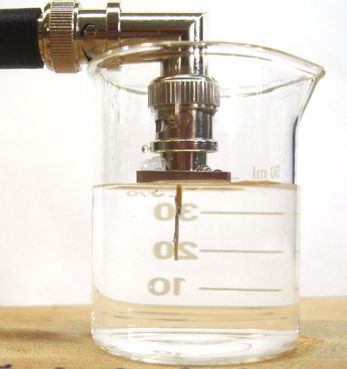
In air, this antenna picks up −61 dBm from a nearby transmitter. We pour water into the beaker as shown above, and received power increases to −49 dBm. We clip the antenna back to 9 mm and we get −54 dBm. We increase to 20 mm and get −52 dBm. We cut back to 15 mm and get −48 dB. See here for measurements of the ideal length of a transmit antenna in water. We measure received power for the 15-mm quarter-wave antenna in water and in air.
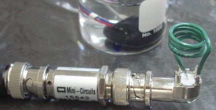
The straight antenna in water acts like a much larger antenn: power can decrease as the transmitter comes near. We make a 15-mm loop antenna and put it on a right-angle BNC plug, so that it rests upon our wood table. This antenna picks up −27 dBm when the transmitter is right over the antenna at a range of a few millimeters. Power greater than −45 occurs if and only if the transmitter is within a few centimeters of the antenna. We raise the 15-mm diameter loop 20-mm off our table and lay a conducting sheet on the table to act as a ground plane. We move our transmitter along the same path as before, but 60-mm above the ground plane. Now we pick up less than −60 dBm everywhere, although we do get more power the closer the transmitter is to the antenna. We move the transmitter around on a stick and find that, almost all the time, power greater than −50 dBm, regardless of orientation and position, indicates the transmitter is within 5 cm of the antenna, and power less than −60 dBm almost always indicates that the transmitter is farther than 10 cm from the antenna.
[15-MAR-16] We make an unterminated 10-turn coil of solid wire 20 mm in diameter and support it 20 mm above a ground plane. Along a platform 60 mm above the ground plane, we move an A3028B mouse-sized transmitter with 30-mm antenna in a 30 ml of water with its antenna loop roughly 20° to the horizontal. We move a distance 30 cm along the platform for various orientations of the transmitter cup about the vertical, so simulate an animal turning around as it moves about a cage.
The coil has rotational symmetry about the vertical axis, but the transmitter does not, hence the variation in reception with transmitter orientation. But we do not expect these graphs to vary as we change the line of motion with respect to the coil. We are usually able to detect the presence of the transmitter 10 cm away. Power at range 0 cm is always greater than power at range 5 cm. An array of such coils on a 10-cm grid could provide location tracking with accuracy ±3 cm, and resolution ±1 cm.
[22-MAR-16] We wind a 3.5-turn 13-mm diameter loop of hookup wire and solder it to a right-angle BNC plug. According to an inductance calculator, this coil should have indutance roughly 160 nH. We combine the antenna with a 3-dB, 50-Ω attenuator, after noting that the power delivered by the antenna increases by 10 dB when we add the attenuator. We place the center of the coil 30 mm above a ground plane made of conducting graphite sheet.
We move the transmitter as before, 6 cm above the ground plane, which is 3 cm above the coil, from position (−15 cm, 0 cm) to (+15 cm, 0 cm) in four orientations. We measure received power every centimeter.
We place the transmitter at the same height, but in five different locations with respect to the fixed receiving coil antenna. At each position, we rotate by 360° in 22.5° steps and record received power.
We see that our receiving coil provides at least 5 dB more power for a transmitter directly above the coil than for a transmitter 5 cm away from the coil, for all orientations and directions.
Suppose we have an array of five receiving coils arranged at positions (0,0), (-5,0), (5,0), (0,5), (0,-5). We have a transmitter directly above the central receiving coil. We measure power received by all five coils. We subtract a threshold of −80 dBm from all our power measurements, this being the power we get when we turn off the transmitter, and so obtain the power above minium for each antenna. We take a weighted centroid of this logarithmic power measurement for each of our sixteen orientations, and so obtain a measurement of position that simulates a transmitter rotating above a receive coil with an array of five coils spaced on a 5-cm grid. The plots below show how the x and y location varies with rotation.
Coils far from the transmitter will have a large effect upon measured position, even if the power they detect is barely higher then our noise level. We introduce into our weighted centroid calculation a power threshold. If a coil power is greater than the threshold, we subtract the threshold to obtain the net power. If the power is less than the threshold, we set the net power to zero. We will use net power in our centroid calculation so as to eliminate the influence of far-away coils. Conversely, a coil directly under the transmitter does not contribute significantly to the overall position measurement, other than to reduce the contribution of the other coils. We remove the central coil measurements of our experiment so as to obtain a position measurement from four coils arranged on a 10-cm square, with the transmitter in the center of the square.
The standard deviation of position is now 15 mm, and we have a step-change in measured position of 50 mm when we go from rotation −22.5° to 0°.
[29-APR-16] We take our 910-MHz SAW Oscillator (A3014SO) and apply its output to an un-calibrated Spectrometer (A3008B) and average power with an early version of the Spectrometer Tool. We use attenuators to vary the power we deliver to the A3008 and check the delivered power with our vector voltmeter.
The slope of the linear part of the graph is 1.00 dB/dBm. The A3008 fails for constant-frequency inputs higher than −20 dB, because the VCO that generates the LO locks its frequency to the RF input and the IF is too low to pass through the IF amplifier's high-pass filters.
[05-OCT-25] We define version A3008E to provide a programmable frequency sweep output. The sweep output on our hand-held and bench-top commercial instruments is too slow for our dynamic tests of demodulation tuning. In the case of tuning an A3038DM-D detector module, we are using a screwdriver to adjust a capacitor and we want to see immediately on the oscilloscope the effect of our movements. We update A3008 documenation.
[06-OCT-25] We open and modify R0201, previously A3008D. We drop C2 to 1.0 μF, which allows the MAX6239 regulator to power up more easily, so it does not latch up. We replace R30 with two diodes in series, using an MA125, so that the DAC reference voltage is close to 1.44 V, and more stable with respect to the value of our +15-V power supply, so as to improve accuracy. We solder 1.0 kΩ to U11-7 and bring this DAC ouput signal through the resistor to a front-panel BNC connector. We reprogram with P3008B01. We define the following opcodes for LWDAQ commands, where the opcode is the four-bit value [DC4..DC1].
| opcode | value | function | |
|---|---|---|---|
| nop | 0 | no operation | |
| set_start | 1 | start frequency := [DC16..DC9] | |
| set_end | 2 | end frequency := [DC16..DC9] | |
| set_dwell | 3 | dwell value := [DC16..DC9] | |
| sel_gnd | 4 | select ground analog return | |
| sel_if1 | 5 | select +0 dB gain | |
| sel_if2 | 6 | select +22 dB gain | |
| sel_if3 | 7 | select +44 dB gain |
The firmware increments the frequency count every (dwell+1) μs starting from the start frequency and ending with the end frequency. A dwell value of zero will lead to no sweep or DAC value writing at all. The dwell and end frequencies reset to 255. The start frequency resets to zero. In this reset state, our dwell time is 256 μs and our sweep takes 65 ms. The kind of sweep we are looking to implement for receiver calibration is 880-950 MHz, which will be around 90 steps. With dwell value of 3, this sweep will complete in 360 μs, so it will be running at 2.7 kHz, which is fast enough.
The new RFPM Instrument operates the A3008E, but is incompatible with the A3008D and earlier versions. So far as we know, there is only one A3008 in the field, at Edinburgh University. We have three in-house. We will update them all and drop support for the A3008A-D in LWDAQ 10.7.5. Because the DAC write is faster, the A3008E is faster at taking spectra. When measuring power, the RFPM does not use a constant LO value, but intead makes use of a sweep of "dither+1" steps with dwell time "dwell+1" microseconds. Our initial values are dither=1 and dwell=3. With the dither in the LO, we eliminate the occasional zeros in power measurement that occur when our source is in phase with our LO. We also increase the width of the spectrometer window. So will increase the capacitors in the IF filter from 100 pF to 200 pF, which will drop the corner frequency of the four-pole Butterworth filter from 1.6 MHz to 0.8 MHz. The window will now be 1.6 MHz. With our dither of 1 MHz, the effective window will be 2.6 MHz, slightly smaller than our original 3.2 MHz. New second page of schematic is S3008C_2.gif. We produce but do not test P3008B02, which drops DAC update time from 1.85 to 0.925 μs and adds a flash of LED2 for each command reception.
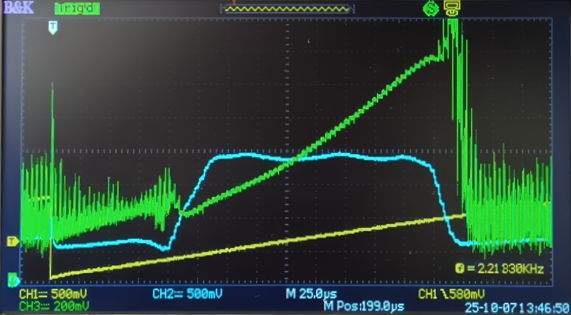
[07-OCT-25] Our P3008B02 is working. We are able to provide dwell times 2 μs to 256 μs. We run the LO output from R0201 through −30 dBm to an A3038DM-D detector module input. We trigger on the falling edge of our sweep's TUNE voltage. We look at the power measurement voltage, P, on the detector module, as well as the demodulator output, D. To configure the sweep we have: sweep start 0x00, sweep end 0x70, and dwell 0x03. With dwell = 3 we have 4-μs dwell time per step, and in the demodulator output we see the eight-bit ADC steps clearly. Each step is roughly 0.8 MHz.
We copy today's version of the RFX.tcl Toolmaker script and adapt for calibration of our A3008E with the help of an RF Explorer spectrum analyzer, which we are controlling and reading out over USB. We create Calib.tcl, a Toolmaker script that steps through a range of DAC values using the RFPM Instrument at each step, and measures for each step the A3008E output frequency and power. We revert to an older LWDAQ and repeat for an A3008D. We plot both calibrations below.
The steps in the calibration are due to the resolution of the hand-held spectrometer. Our objective is to obtain a good calibration of the spectrometers at a reference frequency 915 MHz, combined with an accurate slope. For R0201 we have dac_ref 57.2 cnt and slope 0.824 MHz/cnt. For R0202 we have dac_ref 60.8 cnt and slope 0.772 MHz/cnt.
[08-OCT-25] We improve our calibration code. We increase C14-C17 to 200 pF. We apply first −60 dBm at 905, 910, 915, 920, and 925 MHz and then −30 dBm. We choose our power calibration to correct the −60-dB signals and find that our −30 dBm signals are measured as 3 dB too low. At no point during these measurements do we see any zeros in the power values. Our dither of one count is proving effective at stopping coherence between the signal and the LO.
[21-OCT-25] We upgrade R0202 from A3008D to A3008E. We check our hand-held RFX spectrometer against our SSG-6001-RC and then connect the RFX to our calibration program. We upgrade Q0159 as well. Now we have three completed A3008E and we plot their calibrations all on the same graph below.