Automatic Seizure Detection
Presentation for the Institute of Neurology, UCL
05-FEB-15 (Modified 08-JUL-25)
Kevan Hashemi
Open Source Instruments Inc.
www.opensourceinstruments.com

Voltage vs Time: three types of scaling:
Playback Interval: should suit the patterns we wish to find:
A metric is a real-valued characteristic of the interval, bounded 0 to 1.
Our metrics: power, coastline, intermittency, spikiness, asymmetry, periodicity.
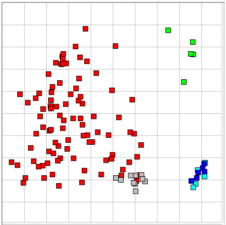
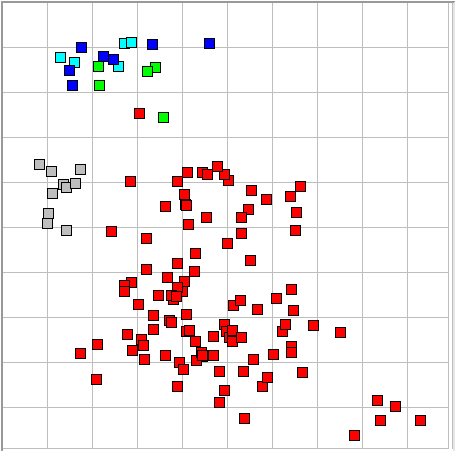
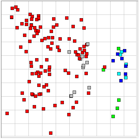
With N metrics, each interval is a point in the N-dimensional unit cube.
With adequate representation, intervals are similar if and only if they are close.
Events of a particular type occupy a connected region of the cube.
With adequate representation, different event regions do not overlap.
The event library is a list of events classified by human eye.
The event library represents the event regions with points within those regions.
Eg: baseline region defined by example baseline patterns.
Eg: ictal region defined by example seizure and inter-ictal patterns.
Suppose we have only one metric, N = 1.
We find we need Q = 4 library events to define baseline and ictal regions.
But find this representation is not adequate, add a metric, now N = 2.
We find we need Q = 16 library events to define baseline and ictal regions.
But find this representation still not adequate, add a metric, now N = 3.
We find we need Q = 64 library events to define baseline and ictal regions.
In general, we may need Q = 4N library events.
For six metrics, Q = 4096.
If event regions are small, may need far fewer.
Experience: with six metrics, ION used hundreds of library events.
We begin with a measure of the signal size, which we call power.
Possible measures: mean absolute deviation, standard deviation, range.
We choose standard deviation for the emphasis it gives to large excursions.
We specify a baseline power for the signal.
We divide the standard deviation by the baseline power.
The result is a dimensionless, calibrated measure of power.
For A3028D, skull screws, rat: baseline = 200 counts = 80 μV rms.
For A3028R, dentate gyrus electrodes, rat: baseline = 500 counts = 200 μV rms.
power_metric = 1 / (1 + (baseline / stdev)), a sigmoidal function of power measure.
power_metric = 0.5 when stdev = baseline.
Coastline: the sum of the absolute steps between samples, divided by the mean absolute deviation of the interval, and passed through a sigmoidal function.
Intermittency: the fraction of coastline generated by the 10% largest steps, and passed through a sigmoidal function.
Spikiness: the average separation of medium, and large peaks and valleys, divided by the signal range, and passed through a sigmoidal function.
Asymmetry: the ratio (max-ave)/(ave-min) passed through a sigmoidal function.
Periodicity: the regularity of large peaks and valleys, and passed through a sigmoidal function.
Normalized Metrics: amplify or attenuate the signal, metric remains unchanged.
These Five Metrics: are all normalized.
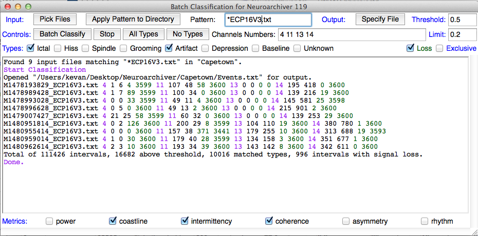
ECP15 is the Event Classification Processor Version 15.
Executed by Neuroarchiver for each channel in each interval.
View and edit with a text editor.
Calls LWDAQ's run-time library to calculate metrics.
Provides a frequency measure also, divide by interval length to get Hertz.
We can omit asymmetry, periodicity, and frequency from characteristics line.
set include_asymmetry 0
set include_periodicity 0
set include_frequency 0
Turn on and off diagnostic display with configuration variables.
set show_intermittency 0
set show_spikiness 0
set show_periodicity 0
set show_frequency 0
set metric_diagnostics 0
Uses baseline powers defined in the Calibration Panel.
Threshold: minimum power for classification, Limit: beyond this distance, an event is Unknown, Normalize: don't use power metric to classify.
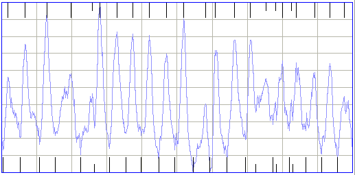
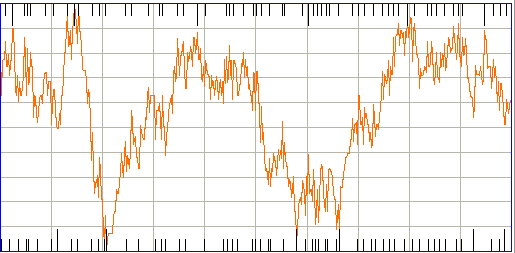
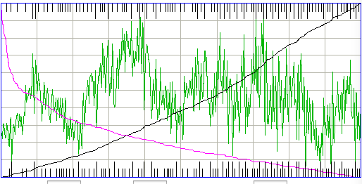
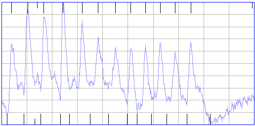
An Ictal Interval with High Coastline and Low Intermittency (Normalized Display).
Note the sharp spikes with rough sides and no obvious period.
We cannot use asymmetry or periodicity to distinguish this interval from baseline.
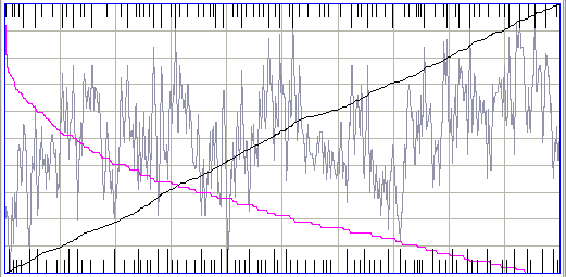
Four-Second Intervals Showing Seizure (left) and Spindle (right).
Asymmetry allows us to distinguish between these two.
Might use asymmetry after first classifying as non-baseline.
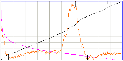
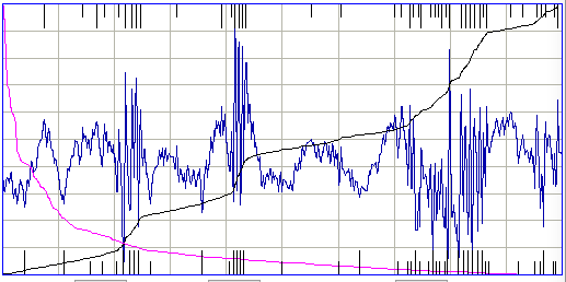
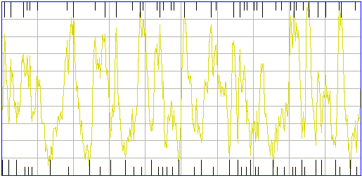
Two Ictal Intervals, one periodic, one not periodic.
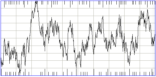
Short black vertical lines are peaks and valleys for spikiness only.
Longer black lines are peaks and valleys used for spikiness and periodicity.
Ideal arrangement: run processor while recording, and never have to re-run.
In practice, may have to re-process the recording.
Table below gives total time to read, reconstruct, and process one channel-second.
Processing is more efficient for longer playback intervals.

Metric calculation in ECP15 takes 1.8 ms/ch/s for 1-s intervals.
Compare to 4.2 ms/ch/s for ECP11V3 and 31 ms/ch/s for ECP1.
Takes characteristics files and event library as input.
Produces lists of events.
Have 16 hours or recording containing 236887 channel-seconds.
Process with ECP15, use Library_02FEB15.txt containing 137 events.
Here is the fraction of ictal-classified events that we agree are ictal.
We vary the classification configurations.
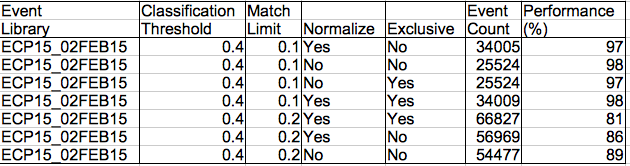
Normalized classification works as well as if we use the power metric.
With only three metrics, 137 events are enough.
False positive rate on baseline intervals is around 0.5%.
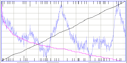 Note: Purple plot shows sorted coastline step size. Black plot shows progression of coastline. Short marks for peaks and valleys used only by spikiness. Long marks for peaks and valleys used by spikiness and periodicity.