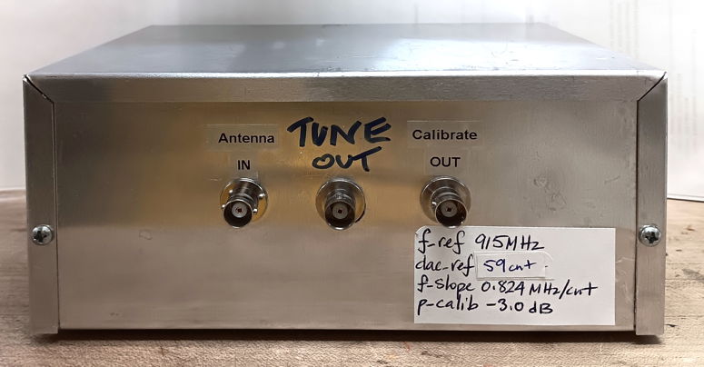
Figure: RF Spectrometer (A3008E) Front Side.
| Description |
| Operation |
| RFPM Instrument |
| Spectrometer Tool |
| Warm-Up |
| Calibration |
| Spectra |
| Design |
[22-JUN-26] The RF Spectrometer (A3008) measures RF power in 3-MHz windows between 850 MHz and 1100 MHz. If you connect the A3008's RF input to an antenna, the A3008 will measure the power spectrum of RF signals arriving at the antenna with 1-MHz resolution and sensitivity 100 pW (−70 dBm). We can use the A3008 to measure average power in the window, peak power in the window, or the power received from a subcutaneous transmitter. To measure the power received from a subcutaneous transmitter, we place the A3008's window at the center frequency of the transmitter. Our subcutaneous transmitters emit a 7-μs burst of power every few thousand microseconds, which is a challenging for a standard spectrometer to detect. The A3008 is designed to detect these burst signals, as well as to measure interference in the 902-928 MHz ISM band.
We use the A3008 to check the output power and spectrum of our transmitters during quality control. We use the A3008 to check that no significant power escapes our faraday enclosures. Another use of the A3008 is to measure ambient interference in the 902-928 MHz band to determine whether the operation of an SCT system is possible within a room proposed for telemetry. Nowadays, however, we can buy hand-held spectrometers that do a better job of measuring ambient intereference. We purchase, configure, and test such hand-held devices on behalf of our customers, and ship them as a component of our telemetry systems under part name and number Hand-Held Spectrometer (HHS1). With these hand-held, battery-powered spectrometers, our customers can check their laboratories for interference so as to diagnose reception problems, should such problems arise. But at the time we designed the A3008, back in 2006, such commercially-available spectrometers were prohibitively expensive, so all our initial measurements of interference power we performed with various incarnations of the A3008.
The A3008 is a LWDAQ device. The LWDAQ software's RFPM Instrument (radio frequency power meter) obtains RF power measurements from the A3008. The Spectrometer Tool gathers these power measurements together into a graph. The A3008 uses an eight-bit DAC to set the TUNE input of a MAX2624 VCO. For DAC values 0 to 255, the VCO output frequency increases from roughly 850 MHz to 1050 MHz. The A3008's RF input is amplified and passes into a mixer, where it is downshifted by the VCO frequency. The resulting IF is low-pass filtered with cut-off frequency 1.5 MHz. The power present at the output of the low-pass filter is proportional to the power present at the A3008's RF input in a 3-MHz wide frequency window centered upon the VCO frequency.
Each spectrometer's amplifiers and local oscillator are slightly different. We account for these variations with calibration constants, which we list on the back wall of the A3008D enclosure. We enter these values into the Spectrometer Tool to obtain ±1 MHZ frequency measurement in the 900-930 MHz band and ±2 dB power measurements in the range −70 to −20 Bm.
| Assembly Version |
Description | Firmware Version |
|---|---|---|
| A | Prototype, no BNC connectors for RF input and LO output. | 1 |
| B | BNC connectors, thermally stable oscillator, ready indicator. | 2 |
| C | Fixed LWDAQ loop-back problems, increased LO power. | 3 |
| D | As C, but in aluminum enclosure. | 3 |
| E | As D, LO sweep function, no warm-up indicator. | 3 |
All versions of the A3008 suffer from a +0.2 MHz/°C shift in measured frequency with ambient temperature. This shift occurs as the VCO frequency changes by −0.2 MHz/°C. We must let the spectrometer warm up for a few minutes to allow it to reach equilibrium. The A3008/C/D flashes its geen power light until the circuit has warmed up. The red light turns on when the A3008B/C/D is in use. The A3008E, however, does not provide a warm-up indicator, because our assumption is that the spectrometer is always powered up and warm.
The A300E can provide a radio-frequency sweep on its Calibration Output. The A3008E firmware allows us to specify a start frequency, a stop frequency, and a step dwell time so that the LO output will provide a fast sweep frequency for tuning, calibrating, and testing devices such as our own telemetry receivers. The amplitude of the calibration output is roughly −3 dBm.
[05-OCT-25] The A3008 consists of a local oscillator (LO), a radio-frequency input (RF), a mixer, a 1.6-MHz low-pass filter, and several intermediate frequency (IF) amplifiers. We obtain the IF by mixing the RF and LO, so that the IF frequency is the difference between the LO and RF. We vary the LO frequency by writing a value 0-255 to the circuit's firmware. We pass the IF through the 1.6-MHz low-pass filter, and so retain only the signal in RF that is in a 3-MHz window centered on the LO frequency. We select one of four amplifications of the IF signal for return to the LWDAQ driver. By digitizing these IF signals, we can determine the power over a range −70 to −20 dBm.
The A3008 amplifies its RF input by 18 dB and feeds it into a frequency mixer for downshifting. The mixer's LO signal comes from a MAX2624, whose output frequency is set by its TUNE input, as shown in the figure below. The IF output from the mixer passes through a 1.6 MHz low-pass filter. The filtered IF signal is the downshifted version of the RF frequencies within 1.6 MHz of the LO frequency. If the LO frequency is 950 MHz, then any RF signal whose frequency is in the range 950±1.6 MHz will emerge from the mixer as an IF signal in with frequency in the range ±1.6 MHz, and so pass through the IF filter.
The A3008 measures RF power in a 3.2-MHz band centered upon its LO frequency. We set the LO frequency using U11, and eight-bit DAC. The DAC can vary the LO chip's TUNE input from 0 V to 2.8 V in steps of 11 mV. The RFPM Instrument allows you to specify the DAC value with its dac_value parameter. When dac_value is 0, the TUNE input will be 0 V. When dac_value is 255, TUNE will be 2.8 V.
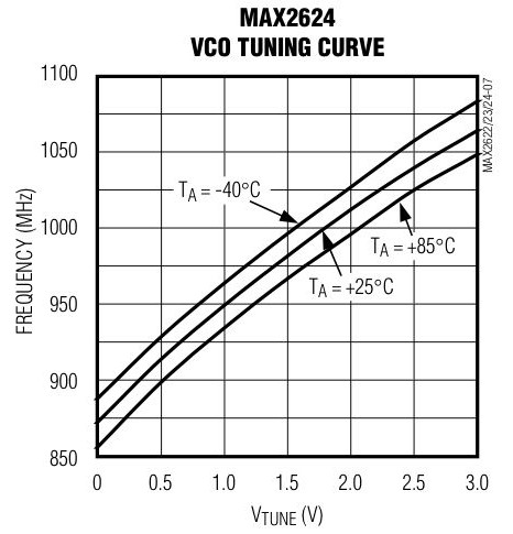
Because eight-bit DAC step causes an 11-mV change in the VCO tuning voltage, and the slope of frequency with tuning voltage is 75 MHz/V, we expect the frequency to increase by ≈ 0.8 MHz per eight-bit count (cnt). We note also the −0.2 MHz/°C change in oscillator frequency, which gives an apparent +0.2 MHz/°C change in the frequency of an external power source. Firmware P3008A01.abl for the A3008A suffers from calibration drift as we take continuous spectra. The VCO warms up as you we use it, but cools down when we don't. Firmware version P3008A02.abl for the A3008B solves this problem by leaving the VCO on all the time. After a five-minute warm-up period, the A3008 is stable.
The filtered IF signal is called IF1 in the schematic. The A3008 amplifies IF1 by ×11 to create IF2, and then amplifies IF2 by 11 to create IF3. The A3008 allows you to select any one of these three IF signals, and also a 0-V reference. The RFPM records all four of these signals using the LWDAQ driver's 8-bit ADC. Each ADC sample takes a minimum of 500 ns. If you set daq_delay_ticks to 0 in the RFPM, the ADC samples will be spaced by 500 ns, so the IF signals get sampled at 2 MSPS. We decrease the sampling frequency by adding 125 ns "delay ticks" to the sampling steps. The daq_delay_ticks parameter is the number of 125-ns delays you would like added to each 500-ns ADC sample. The daq_num_samples parameter tells the RFPM how many samples to take of each IF signal. We obtained most of the graphs below with 20 delay ticks and 10,000 samples. The sample period is 3 μs, the sample frequency is 333 kHz, the time per display division is 3 ms, and the total observed interval is 30 ms.
The RFPM Instrument plots all IF signals that do not exceed the dynamic range of its display. It returns the peak-to-peak voltage it obtains from each of its four IF channels. The Spectrometer Tool translates these peak-to-peak voltages into RF power in decibels, and plots the power in its graph window. The spectrometer provides its own help with its Help button.
[22-JUN-26] Plug the A3008 into the LWDAQ. The green light on the back of the enclosure should turn on steadily or start flashing, depending upon your version of the A3008. If the green light does not illuminate, uplug and plug in the connector again. Wait for a few minutes before using the spectrometer. We need to let it warm up. If we use the A3008 before it's warm-up period of roughly four minutes has passed, its frequency calibration may be off by up to 4 MHz. Other than this frequency error, however, the A3008 will work perfectly well immediately.
For a plot showing how the A3008B's on-board oscillator frequency varies during warm-up, see below. Open the RFPM instrument in your LWDAQ software. Set it up to acquire from your A3008. You will need to set the daq_ip_addr and the daq_driver_socket. Press Acquire. You should see waveforms on the screen, and with each acquisition, four numbers appearing in the text window, as shown below. Whenever you press Acquire, you should see the yellow ACTIVE light on the A3008B flash.
The RFPM Instrument provides three types of power measurement: average or maximum. When you set analysis_enable to 1, the result string contains the range over which each trace varied during the its measurement period. The range is the maximum value minus the minimum value. With analysis_enable set to 2, the result is the standard deviation of each trace. The former gives us peak-to-peak voltage, the latter is rms voltage. If the RFPM sees a sinusoidal waveform, the peak-to-peak voltage will be 2.8 times greater than the rms voltage.
The dac_value sets the A3008's LO (local oscillator) frequency. The A3008B mixes the LO with the RF input to produce an IF frequency that we low-pass filter with a cut-off of 1.6 MHz. The ±1.6 MHz pass-band of the low-pass filter gives the A3008 a 3.2-MHz pass-band centered upon the LO frequency. What you see in the display of the RFPM is whatever signal is present within this 3.2-MHz passband. The RFPM obtains three traces from the A3008, each with higher gain than the last. It displays only the traces that are not saturated in intensity. The following table lists the four traces. The gains we give in the above table are voltage gains with respect to IF1 in the schematic).
| Trace | Color | Gain |
|---|---|---|
| 0 | red | 0 |
| 1 | green | 1 |
| 2 | blue | 11 |
| 3 | orange | 121 |
The daq_num_samples parameter sets the number of samples of each signal (gains 0, 1, 11, and 121) the RFPM analyzes and displays. With daq_delay_ticks = 0, the samples will be recorded with a period 500 ns (2 MSPS). With daq_delay_ticks = 1, the samples will be recorded with period 625 ns, and so on, with the period increasing by 125 ns for each increment of daq_delay_ticks.
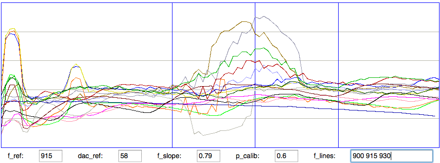
[22-JUN-26] The Spectrometer Tool uses the RFPM Instrument to measure power at a range of frequencies. Before you use the Spectrometer Tool, configure the RFPM Instrument to read values from your Spectrometer (A3008) device. The power is displayed in dBm. The frequency range is defined by count_min and count_max in the Configuration Panel. These are integers in the range 0-255, corresponding to the eight-bit parameter dac_dac_value in the RFPM Instrument. The power range is from power_min to power_max. The Spectrometer draws vertical lines upon the plot to mark the frequencies listed in f_lines. We specify these frequencies in megahertz.
Each spectrometer has a slightly different relationship between its DAC control number and its LO frequency. In f_ref we enter a reference frequency in megahertz and in dac_ref we enter the DAC value that causes our spectrometer device to generate this frequency. In f_slope we enter the slope of frequency with DAC value in megahertz per count. In p_calib we enter a power offset to correct the raw power measurement from the Spectrometer hardware. In the calibration section below, you will find values for these three calibration constants for your A3008 circuit.
Open the Spectrometer Tool from the Tools menu. Press Scan. Assuming you have set up the RFPM Instrument correctly, the spectrometer will begin to plot a spectrum. Press Repeat and it will monitor one frequency. To plot the spectrometers noise, select the Average measurement type and unplug the A3008's antenna. Noise is generated by the A3008 itself, but also invades the A3008 amplifier from outside. You may see peaks in your spectrum that correspond to local interference. In the plot above, we see peaks at 926 MHz that are local interference.
With the Save and Load buttons, you can save and load spectra as text files. The raw Spectrometer data we link to in the sections below is data we saved to disk in this way. You can download it, look at it with a text viewer, and read it into your own Spectrometer to see the graphs. The Spectrometer plots data in its active graph. You can clear the active graph with the Clear button, and all graphs with the Clear All button. Each graph has its own color, and each graph is named after a letter. When you obtain a new point in a graph that duplicates a previously-existing step value in the same graph, the Spectrometer deletes the previous graph point.
You can turn on and off the cursor with the cursor check box. The horizontal grid lines you can adjust with step_min, step_max, and step_div. By default, the Spectrometer measures SCT power, but you can instruct it to measure average or peak power with the Measurement option menu. The SCT power measurement differs slightly from the peak power measurement in that the SCT spectrum is spread out, so the 3-MHz window of the A3008 does not detect all its power. We add roughly 2 dB to the peak power measurement to obtain the SCT power measurement. You can add frequency lines with the "Frequency Lines" entry box. You specify each line with a single frequency in megahertz.
[05-OCT-25] We disconnect our A3008B from power and let it cool for an hour. We take the local oscillator (LO) output from our A3008B and feed it into the RF input of a mixer. We use our 868-MHz SAW Oscillator (A3014SO) as a source of LO for the mixer. We measure the period of the intermediate frequency (IF) on our oscilloscope. We plug power into the A3008B, and set its frequency-control DAC to 10 counts immediately. We measure the A3008B's LO frequency by adding 868 MHz to the intermediate frequency we observe on the oscilloscope. By this means we are able to plot LO frequency versus time.
A four-minute warm-up period is adequate for 1-MHz calibration accuracy. According to this plot, the temperature coefficient of the MAX2624 frequency is around −30 MHz / 125°C = −0.25 MHz/°C. A 4°C change in room temperature causes a 1 MHz error. The A3008D and subsequent versions leave the internal LO running so long as the device is connected to LWDAQ power. We do not have to wait for the device to warm up because it should always be warm and stable.
[22-JUN-26] The A3008B and later provide a BNC socket with approximately +3 dBm of its internal LO signal. This allows us to calibrate the LO with respect the eight-bit DAC values we use to set its tuning input voltage. For this calibration, we need either a spectrum analyzer or an accurate local oscillator and a mixer. In our original calibrations, we used a ZAD-11 mixer and a home-made 910.3-MHz SAW Oscillator (A3016SO). Nowadays, we connect the calibration output to a spectrum analyzer and measure its frequency versus RFPM Instrument daq_dac_value. The slope of this line, and its value at 915 MHz provide our frequency calibration parameters f_slope (MHz/cnt), dac_ref (cnt at reference frequency) and f_ref (reference frequency in MHz).
We apply a subcutaneous transmitter signal of known power to the antenna input and measure the peak power of its spectrum. We adjust p_calib in the Spectromater instrument until the peak power measurement equals the subcutaneous transmitter burst power output.
The LO output power of the A3008 is constant to ±0.5 dB from 875-1050 MHz, but varies by ±3 dB from one circuit to the next. When we mix the LO with a nearby frequency, the IF shows phase nnoise of ±75 kHz. The fluctuations in frequency are due to noise on the input of the VCO that generates the LO on the Spectrometer circuit. These fluctuations are beneficial to the spectrometer because they prevent loss of power measurement when the LO and RF signals have the same frequency. When the IF is below 100 kHz, it is attenuated by the high-pass filters in the IF amplifier. Because the LO fluctuates by 150 MHz, we are certain to obtain a power measurement even when the average RF frequency is equal to the average LO frequency.
Fluctuations in the LO frequency prove to be so be so beneficial that the RFPM Instrument deliberately introduces them into the LO output by instructing the A3008 to dither between two frequencies one DAC step apart. By this means the fluctuations are increased to ±400 kHz. Another benefit of the fluctuations is that they stop the LO of the A3008 from generating bad messages in a nearby Octal Data Receiver (ODR). Only the A3008E and later versions of spectrometer firmware provide this dither.
[05-OCT-25] The 902-928 MHz Industrial, Scientific, Medical (ISM) frequency band is recognized for unlicensed use in North America, South America, and the UK. In countries where the 902-928 MHz band is reserved for the exclusive use of license-holders, our faraday enclosures ensure that no significant RF power is radiated by our SCT system, thus making sure we do not violate local regulations. The regulations governing the 902-928 MHz band have evolved in the years since we first chose it for our SCT telemetry in 2005. The band is still recognised for unlicensed transmitters up to 1 W in North and South America. But in 2013, the FCC granted a private company a license to transmit up to 30 W in the USA. A 30-W transmitter less than 10 m from one of our recording systems will disrupt reception. But such proximity should be easy to avoid.
In Europe, the UK recognises the 902-928 MHz band for unlicensed transmitters up to 1 W, but they have granted mobile phone companies license to use the same band with base stations transmitting up to 3000 W effective radiated power. An SCT telemetry system directly in the path of such a base station transmission will be disrupted at ranges less than 100 m. Mobile base stations tend to be over twenty meters above the ground, mounted on towers or the sides of tall buildings. The upper floors of neighboring buildings receive the most power from such base stations. Near base stations, lower floors are better than upper floors, and basements are best.
In the paragraphs below we present spectra we and our customers obtained with A3008 spectrometers in various locations around the world. During our earliest measurements, we were still considering which frequency band to use, but we soon settled upon the US 900-MHz ISM band.
[01-MAR-06] Below is a detail from the low-frequency end of our outside spectrum on a hill in Waltham, MA, near Boston.
We have a peak in the blue curve at 900 MHz and 1000 MHz. We have orange vertical markers at 930 MHz, 950 MHz, and 970 MHz. To match the outside spectrum with the blue peaks and the orange vertical markers, we must shift it by 7 frequency steps to the right. We obtain the following table of interference power in various frequency bands. We quote power relative to the bottom of our spectral graphs.
| Band | Power Density | SCT Range |
|---|---|---|
| 875-902 MHz | +30 dB | 60 cm |
| 902-928 MHz (ISM) | +15 dB | 400 cm |
| 928-945 MHz | +30 dB | 60 cm |
| 945-960 MHz | +15 dB | 400 cm |
| 960-990 MHz | +10 dB | 600 cm |
| 990-1050 MHz | +15 dB | 400 cm |
The +30 dB power at 930 MHz explains why we could not operate A3006 transmitters outside at any range. The weakness of the A3006 is that it does not transmit power in the A3005 receiver pass band during zero bits, so that any ambient power above about +15 dB will saturate it during zero transmissions, and so give false zeros. With the new A3009 transmitters, and modified A3005 receivers, we will be transmitting zeros and ones within the receiver pass band, so we expect to be able to dominate the interference by bringing the transmitter close enough to the receiver.
Below we see the spectrum recorded by the A3008 for an active A3006 Subcutaneous Transmitter at ranges 60 cm and 600 cm in the basement lab. Note that the spectrum extends up to 1050 MHz. This may be a failure in the A3008's ability to reject frequencies outside its current selected band, or it may be that the A3006's spectrum really does extend up into the 1050 MHz band. We have no way at the moment to distinguish between the two possibilities. Note that the ratio of the peak power at 950 MHz is roughly 20 dB (×100), which is what we expect with an increase in range of ×10.
For reliable data recording by a dual receiver, we believe the SCT power must be at least +10 dB greater than the interference. This minimum power sets the maximum range at which the SCT can operate. With +10 dB of interference, the SCT power must be >20 dB, which is the case for ranges less than 6 m. With +30 dB of interference, the SCT power must be >40 dB, which it is at ranges less than 60 cm. When we step inside the doorway, the SCT ranges improve because of the shielding provided by the building.
| Band | Power Density | SCT Range |
|---|---|---|
| 875-902 MHz | +20 dB | 300 cm |
| 902-928 MHz (ISM) | +8 dB | 700 cm |
| 928-945 MHz | +20 dB | 300 cm |
| 945-960 MHz | +8 dB | 700 cm |
| 960-990 MHz | +8 dB | 700 cm |
| 990-1050 MHz | +8 dB | 700 cm |
The interference in our basement laboratory, ignoring that coming from the SCT dual receivers themselves, is as follows.
| Band | Power Density | SCT Range |
|---|---|---|
| 875-902 MHz | +10 dB | 600 cm |
| 902-928 MHz (ISM) | +8 dB | 700 cm |
| 928-945 MHz | +10 dB | 600 cm |
| 945-960 MHz | +8 dB | 700 cm |
| 960-990 MHz | +8 dB | 700 cm |
| 990-1050 MHz | +8 dB | 700 cm |
We provide the above table as a reference, because we have observed the reception at range 6 m to be stable with a dual receiver in our laboratory. It is clear that here in Waltham, operating in the 1000-1050 MHz would be perfect. But the band 960 MHz to 1215 MHz has been reserved for Aeronautical Navigation. Transmitting 300 μW in this band within the confines of a laboratory would have no effect upon aeronautical navigation. Within five meters of the laboratory's external walls, the Subcutaneous Transmitter's signal will be beneath thermal noise. We could ship transmitters in metal boxes, or wrapped in foil. If the transmitter turned on by impact or magnetic field, no measurable power would escape the wrapping.
We would prefer, however, to operate in the ISM band, which is free for anyone to use. The ISM band appears to be the 26-MHz range between the peaks seen in the outside spectrum. We cannot be exactly sure of the frequencies to within a MHz, but we are confident to within 5 MHz. Certainly, it's worth trying the ISM band here in the United States.
[02-MAR-06] A few weeks ago, we recorded the following spectra in and outside our laboratory at 8 pm. The outside temperature was -2 °C. We recorded the red spectrum just inside the doors, where it was 15 °C. We see the same spectrum as outside, but attenuated by 10 dB, and shifted up by five frequency steps, or roughly 3.5 MHz.
The blue trace we obtained ten minutes later in the basement laboratory, with no SCTs turned on, but the SCT dual receiver with their 1-GHz local oscillators turned on. The temperature in the laboratory was 19 C. We see signs of the same features at around step 60 as we saw outside, but shifted up by seven frequency steps, or roughly 5 MHz. The VCO tuning curve above shows a 25 MHz drop in VCO frequency with a 125 °C rise in temperature. That's −0.2 MHz/°C. With our 21 °C increase in temperature from outside to inside, we expect our LO frequency to decrease by roughly 4 MHz. We observe roughly 5 MHz. We took another spectrum with our SCT dual receivers unplugged. The two peaks at 1 GHz (step 163) and 900 MHz (step 34) disappeared.
[10-MAR-06] We obtained the following spectra using our Modulating Transmitter (A3001A). We drive its TUNE input with a square wave that switches from 1.1 V to 1.4 V at frequencies 200 kHz, 2 MHz, 5 MHz, and 10 MHz.
We see the Bessel function curves predicted by theory when the modulation bandwidth is comparable to the separation of the two frequencies. In our case, the two frequencies are separated by 30 MHz, and we start to see the Bessel function at a modulation frequency of 5 MHz.
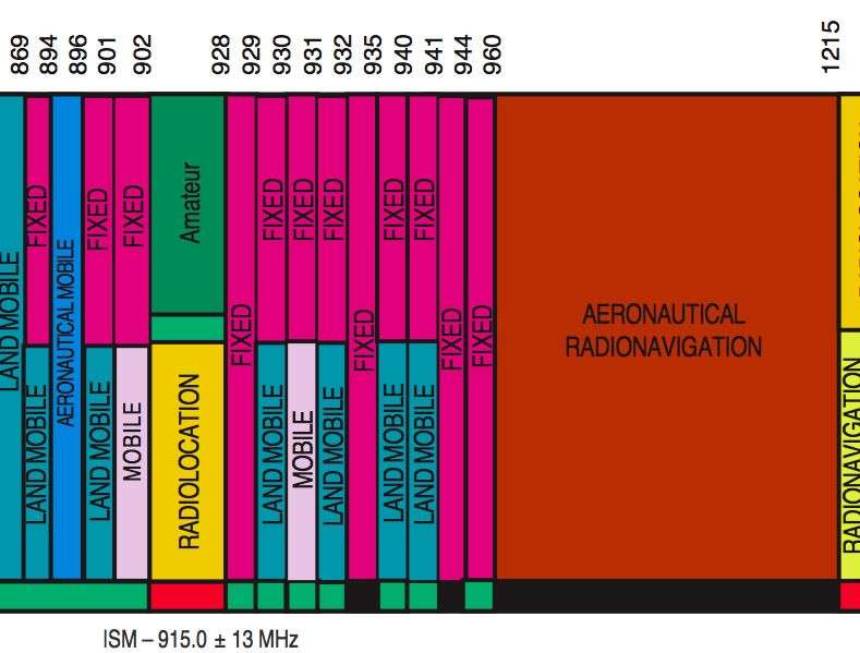
[31-MAR-06] It appears that the ISM band is respected in the UK also, as shown here. They describe the ISM band as "Fixed, Amateur".
These are the spectra from Matthew Walker's laboratory and recording room, recorded by Matthew Walker himself. The recording room is where the rats with implants will live. The laboratory is outside his office. There is broad interference across the entire frequency band in the laboratory. When someone turns their mobile phone on, the spectrum rises by 10 dB, and becomes erratic. We suspect that we are seeing the mobile phone's spurious power emissions, which may be transient. The Spectrometer measures the maximum received power in its measurement interval, not the average power. When we look at the two laboratory spectra without local mobile phone interference, we see what looks like the sum of many mobile phones transmitting in the same broad way, in neighboring buildings. In the recording room, we have three spectra from three different locations. They show residual power in the Fixed Mobile 5.317A band, 942 MHz - 960 MHz. From the location of this band, we think we can say that the vertical black lines in our plot lie upon 20-MHz boundaries. If that's the case, then the peaks to the left is at 930 MHz, in another fixed mobile band. Below that we have several power peaks in the range 910 MHz to 925 MHz. The power in these peaks is approximately equal to the power we record from an A3006 SCT at range 6 m. At range 3 m, an A3009 SCT would dominate the interference. We should be able to operate in the ISM band in Matthew's recording room at ranges less than 3 m.
The above figure shows interference power peaking about 10 dB higher than our signal power at 1 m, even in a favorable orientation. The 902-928 MHz ISM band must be in use for some unlicensed devices more powerful than our own, or France does not respect the band. The operating range of the transmitter in this interference is only a 10 cm.
[31-MAY-07] These following spectra are taken with the new A3008B after we calibrated its ISM-band frequencies to 1-MHz accuracy, as described above.
The red trace is with the RF input terminated with 50 Ω. The green trace is with a Loop Antenna (A3015A) connected to RF with a 96" coaxial cable, but all of our own sources of ISM-band power off. We leave the Loop Antenna connected for the rest of the spectra. The blue trace is with our 910-MHz +12-dBm SAW Oscillator (A3014SO) turned on, with a 75-mm wire as an antenna, place 50-cm from the spectrometer antenna. You can see the large bump corresponding to the 910-MHz, and many other bumps. For the orange trace we insert a 20-dB attenuator in the antenna line. For the yellow trace, we turn off the 910 MHz and turn on a Subcutaneous Transmitter (A3013A) and place it 50-cm from the Spectrometer antenna. For the purple trace, we move this same transmitter to a range of 5 m.
[09-APR-09] Subsequent work on the spectrometer reveals that its noise floor is at −80 dBm. This floor is visible on the right side of the plot above: its is the green straight line. The interference power rises to a peak of −51 dBm, with another broad peak at −60 dBm. The spectrometer has a measurement bandwidth of 3 MHz, so we can calculate the total interference power in the 900−930 MHz band by dividing the band into ten 3-MHz sections and adding the power together. We arrive at roughly −48 dBm total interference in the band. In a separate experiment, we measured the interference power in our basement laboratory in Boston with our Demodulating Receiver (A3017), and found it to be −68 dBm. Our operating range in there is 100 cm. With 20 dB more interference, our operating range will be ten times less, or 10 cm.
[15-APR-09] Today reception was good in the ION animal laboratory. The interference spectrum, taken by Pishan with A3008B number 001, shows less power than the one Matthew obtained in 2006.
[22-JAN-10] We obtained the following spectra in the Children's Hospital Boston basement, in the Operating Room (OR) and the Animal Room (AR). We also show spectra obtained the day before outside in Waltham.
[25-JAN-10] We obtained the following spectra at the OSI office on Moody Street, Waltham.
[20-SEP-13] We receive the following spectrum from her animal laboratory in Edinburgh.
Above 927 MHz, interference power is -45 dBm in each 3-MHz window examined by the spectrometer. Iris is using an A3015B antenna, which contains a 3-dB attenuator, so actual power is around -42 dBm. In 927-930 MHz, where we are sensitive, there is -42 dBm of power. This is great enough to require a faraday enclosure for reliable reception with only one receiving antenna.
[11-NOV-13] We take our first spectrum at our new OSI office on Pratt Ave.
The peak at 926 MHz is −46 dBm. Our Moody Street office has a peak at 926 MHz also, but it is only −60 dBm. Reception in the Bratt Avenue office is not robust even at range 20 cm.
[06-MAR-14] We take a spectrum at MRC Harwell, reception building. We equip the A3008B with an A3015C damped loop antenna.
There appears to be no interference in the 900-930 MHz band. We obtain robust reception with one antenna up to 50 cm.
[25-MAR-16] We take the following spectra in the OSI basement office in Waltham, MA.
Isolation provided by the FE2F is around 26 dB. Interference outside the faraday enclosure is centered on 926 MHz and −48 dBm. Previous measurements show reception of up to −45 dBm in other office locations. Other than this peak, there is no measurable interference. The same three transmitters emit roughly 6 dB more power when immersed in 200 ml of water. From the above graphs, the temperature coefficient of the A3028E center frequency is −0.2 MHz/°C, which agrees with the data sheet.
[30-JAN-17] Spectra from Philipps University, Marburg, showing RF power inside and outside faraday enclosures with subcutaneous transmitters running within the enclosures. We see no sign of significant interference within the 900-930 MHz band.
[27-JUL-17] We receive the following spectra Edinburgh University, where they recently moved their SCT recording system from one room to another on the top floor of their CCNS building. Room A is the original room, from which we obtained spectra in 2013.
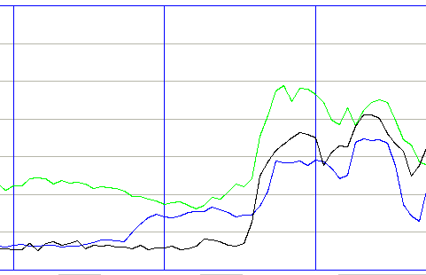
Peak interference power in the Corner Room is −41 dBm (80 nW) outside the Faraday enclosure and −61 dBm (800 pW) inside. In the edge room, meanwhile, we have peak interference in 900-930 MHz of −54 dBm (4 nW). The spectrometer measures the power in a 3-MHz band, while the interferene we see above spans 6 MHz at the top of the 900-930 MHz range our SCT receivers are sensitive to. Thus we estimate the total interference power is equivalent to a single frequency of 160 nW outside the enclosure in the Corner Room, 1.6 nW inside the enclosure in the Corner Room, and 8 nW outside in the Edge Room. Reception from implanted SCTs is reliable only when interference outside the enclosure is less than 40 nW. Thus we expect reception to be unreliable in the Corner Room, and indeed it is: for 30% of the time, reception is less than 80%.
| Number | Measurement |
|---|---|
| 0 | Corner room, outside enclosure, average power |
| 1 | Corner room, outside enclosure, average power |
| 2 | Corner room, inside enclosure, average power |
| 3 | Corner room, inside enclosure, average power |
| 5 | Corner room, inside enclosure, SCT power |
| 6 | Corner room, inside enclosure, average power |
| 8 | Edge room, inside enclosure, average power |
| 9 | Edge room, outside enclosure, average power |
| 10 | Corner room, outside enclosure, average power |
The original recording room was the Edge Room, with one outer wall on the top floor of the CCNS building. The new room is the Corner Room, directly opposite another taller building with three mobile phone base stations. According to a map of the local base stations, the nearest is 60 m away from the Corner Room, with only the outer building wall as an attenuator. The Edge Room is 80 m away with three attenuating walls. The interference power we see in all three traces above correspond to the 925-960 MHz downlink band of the 900 MHz GSM network.
[05-OCT-25] For design files and a history of the development of the A3008, see its D3008 design page.