[14-FEB-26] Our telemetry sensors and stimulators are battery-powered devices designed for use in small animals. Some are designed for subcutaneous implantation, some for intraperitoneal implantation, and some to mount upon an animal's head. All varieties use the same frequency-modulated, microwave messaging protocol to transmit their telemetry data. All varieties capable of receiving wireless commmands do so with the same amplitude-modulated, microwave messaging protocol. Animals with implanted transmitters can be co-housed. Animals with head-mounting transmitters can, in principle, be co-housed, but in practice the animals will destroy one another's head-mounted sensors.
Our telemetry receivers record signals from all telemetry devices within range of their antennas. Combined telemetry receivers and command transmitters use the same antennas to both record and control all devices within range of their antennas. Our telemetry sensors amplify, digitize, and transmit high-fidelity biometric signals, intracranial electroencephalogram (iEEG), local field potential (LFP), electrocorticogram (ECoG), electromyogram (EMG), electrocardiogram (ECG), electrogastrogram (EGG), blood pressure, and body temperature. They permit the study of epilepsy, spreading depolarization, spreading cortical depression, sleep disorders, gastric slow waves, and heart disease in animals as small as juvenile mice. Our implantable stimulators provide wireless electrical and optical stimulation to accompany biopotential recordings.
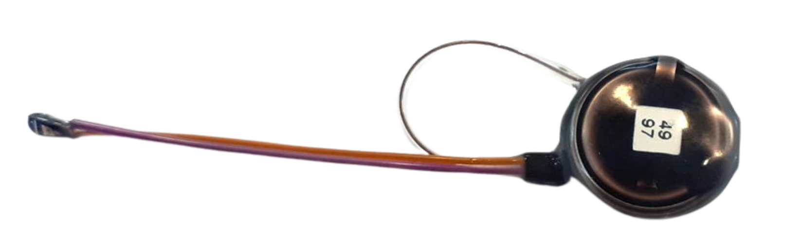
Our Subcutaneous Transmitters (SCT) are battery-powered telemetry sensors designed for implantation beneath the skin of mice and rats. Animals with implanted SCTs can be co-housed. We turn them on and off with a magnet. Each SCT amplifies, digitizes, and transmits one to four biopotentials. Some measure temperature as well. All versions sample biopotentials with an on-board sixteen-bit analog-to-digital converter. Features such as input dynamic range, low-frequency cut-off, high-frequency cut-off, sample rate, device mass, operating life, lead length, and lead terminations are chosen by the customer to suit their needs, subject to the constraints of current consumption and battery capacity. Typical input dynamic ranges are 30 mV, 120 mV, and 300 mV. The pass-band of a sensor is the range of frequencies it can record faithfully. The passband of our SCTs can occupy any portion of 0.0-640 Hz. One of the most common pass-bands is 0.2-80 Hz. Another popular pass-band is 0.0-160 Hz. Less common is 0.2-640 Hz. Sample rates range from 64-2048 SPS (samples per second). Operating life can be as short as seven days and as long a two years. Our smallest transmitters have mass 1.5 g and are suitable for implantation in young mice. Our largest are 14 g and suitable for implantation in large rats. The SCT battery cannot be replaced, but operating life can be long enough to permit several uses of the same device.
Our Head-Mounting Transmitters (HMT) attach to an Electrode Interface Fixture (EIF) cemented to the skull of an animal. These devices are similar to our SCTs in that they amplify, digitize, and transmit one to four biopotentials. But they have no on-off switch. Before the HMT battery exhausts itself, we remove the HMT and replace it immediately with another. Later, we remove the near-exhausted battery from the first HMT, and when the second HMT has nearly exhausted its battery, we use the first with a fresh battery to replace the second. In this way, we can, in principle, record indefinitely from one animal. Although our telemetry system supports recording from multiple HMTs in the same animal cage, doing so is impractical because mice and rats will pull the HMTs off the heads of their cage-mates.
Our Implantable Inertial Sensors (IIS) transmit acceleration and rotation. They turn on and off with a magnet. The IIS is designed for implantation in animals or attachment to fish. When implanted in animals, the animals can be co-housed.
Our Implantable Stimulator-Transponders (ISTs) hibernate when placed next to a magnet, but otherwise are activated and controlled by amplitude-modulated microwaves. These amplitude modulated commands are distinct from the frequency-modulated messages transmitted by our implantable devices, but they use of the same telemetry antennas. Animals implanted with ISTs can be co-housed. The IST will provide electrical stimulation through its stimulus leads, or it can be combined with an Implantable Light-Emitting Diode (ILED) to provide optical stimulation.
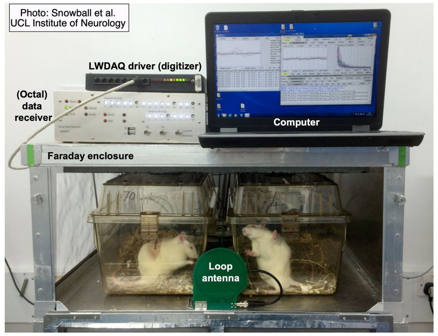
A Telemetry System at the very least consists of one or more telemetry sensors, a telemetry receiver, and a data acquisition computer running our LWDAQ Software. Most telemetry systems include one or more Faraday enclosures to isolate the system from ambient microwave interference. Some telemetry systems use a combined telemetry receiver and command transmitter in order to operate our implantable stimulators as well as receive from our implantable sensors. The computer and receiver communicate with one another over TCPIP messages. A coaxial antenna receiver gathers telemetry signals with telemetry antennas on the end of coaxial cables. An antenna array receiver gathers telemetry signals with antennas fixed in an array on a platform.
The Animal Location Tracker (A3038, or ALT) is an antenna array receiver that we connect to Power over Ethernet (PoE). The Telemetry Control Box (TCB) is a coaxial antenna receiver. The discontinued Octal Data Receiver (ODR) is a coaxial antenna receiver that requires a LWDAQ Driver to provide power and an Ethernet interface.
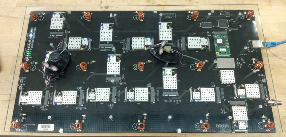
The ALT requires no external antennas. It will record from whatever transmitters share its Faraday enclosure, or we can configure the ALT to record from only certain transmitters. The ALT provides, in addition to telemetry signals, a measurement of the position of each transmitter on its array of detector coils.
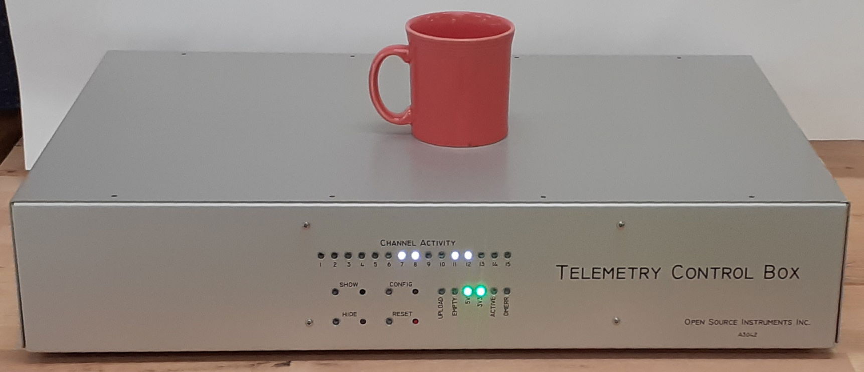
The A3042A-16 Telemetry Control Box (TCB) provides sixteen antenna inputs to which we can connect up to sixteen A3015 Telemetry Antennas for telemetry reception. The A3042B-16 TCB provides sixteen antenna connections that act both as telemetry receivers and command transmitters for radio-controlled implants. We can place four such antennas in each of four bench-top Faraday enclosures. Or we can place sixteen antennas in a single Faraday canopy that encloses a shelf or rack. In each case, we can record from dozens of animals.
Our Faraday enclosures isolate the telemetry system from ambient microwave interference. Before investing in one of our telemetry systems, send us your animal laboratory's latitude and longitude so we can check for nearby mobile phone base stations. We will consult a global database to see if there are any base stations near your building. We recommend you do not attempt to operate our telemetry system within 50 m of a 6-kW base station or within 20 m of a 1-kW base station. Our telemetry system uses the 902-928 MHz band for communication. This band is one of the unlicensed Industrial, Scientific, and Medical (ISM) bands in the United States, so we are free to transmit power in this band without a license. But in other countries this same band may be assigned for licensed use, in which case our Faraday enclosures serve two purposes. Not only do they isolate the telemetry system from local, licensed microwave interference, they also prevent the telemetry system from radiating microwave power in any licensed frequency band.
Our SCT (Subcutaneous Transmitters) and HMTs (Head-Mounting Transmitters) will monitor intracranial electroencephalogram (iEEG), local field potential (LFP), electrocorticogram (ECoG), electrocardiogram (ECG), electromyogram (EMG), and electrogastrogram (EGG) at frequencies down to 0.0 Hz and up to 640 Hz. We currently have three families of SCT in production, each of which is available in a large number of variants. Every active input on an SCT or HMT produces a stream of telemetry samples with a particular identifying channel number. We refer to a transmitter with two active inputs as a two-channel transmitter. We have two-channel transmitters that will record iEEG and ECG in mice. We have three-channel transmitters that will record EMG in one location on the neck of a rat and iEEG in two locations on the brain. We have four-channel transmitters that will record iEEG, EMG, ECG, and EGG simultaneously in rats. All our SCTs can be configured for AC recording with passband down to 0.2 Hz, or DC recording with passband down to 0.0 Hz. For example recordings, see our Example Recordings page.
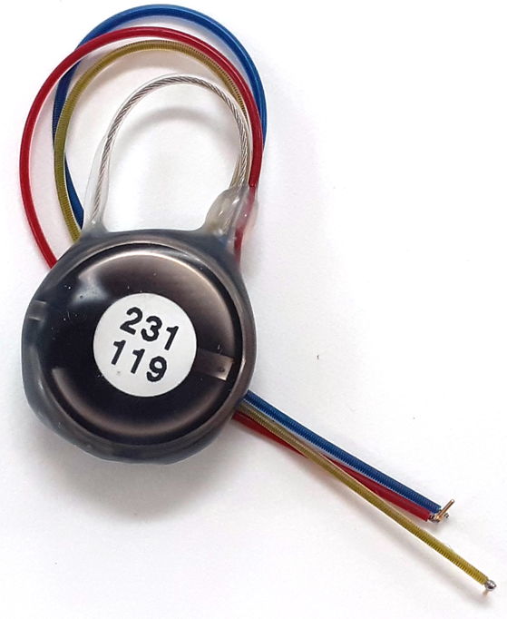
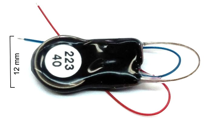
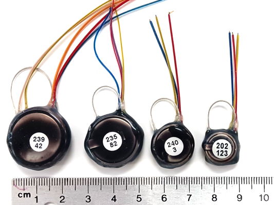
The A3048 SCTs are a family of single-channel sensors. The A3048P is our smallest sensor with mass 1.5 g and thickness 3.7 mm. The A3048S is slightly larger, with mass 1.9 g. The A3048S2, with its 0.2-80 Hz passband and 256 SPS sample rate, is our most popular iEEG sensor. The A3049 SCTs are a family of one and two-channel sensors. The smallest A3049 is the A3049W with mass 2.0 g. The largest A3049 is the A3049L with mass 14 g. The A3047 is a one to four-channel SCT that incorporates its own temperature sensor. The mass the A3047A is 6.7 g. The A3040 HMTs are a family one to four-channel head-mounting sensors with mass 2.2 g. All these families of SCTs and HMTs can be configured for both AC and DC recordings.
The primary purpose of our telemetry system is to record biopotentials continuously for weeks at a time, to provide intermittent stimuli for weeks at a time, and to analyze the recordings automatically. When recording iEEG in epileptic animals, we want to count seizures in tens of thousands of hours of recording. Our two-channel transmitters can be equipped with either three or four leads. In the three-lead configuration, the two biopotential inputs share the same reference potential. These devices are ideal for recording iEEG in two locations using the cerebellum as the reference potential. In the four-lead configuration, each input has its own reference potential. These devices are ideal for recording two distinct biopotentials, such as iEEG and ECG. Our four-channel transmitters can be equipped with eight leads, so that each input has its own reference potential. These devices are ideal for measuring four distinct biopotentials, such as iEEG, ECG, EMG, and EGG.
We assemble every set of telemetry sensors to suit each customer's requirements. To record spreading depolarization and all ictal activity with the same input, we set the pass-band to 0.0-160 Hz and the dynamic range to 120 mV. To count epileptic seizures with the greatest accuracy and precision, we set the pass-band to 0.2-80 Hz and the dynamic range to 30 mV. To record EGG we set the pass-band to 0.0-20 Hz. The bandwidth of a sensor is, strictly speaking, the width of the pass-band. But we use the term "bandwidth" to mean the high-frequency cut-off of the pass-band. Our low-frequency cut-off is so much smaller than the high-frequency cut-off, that the bandwidth and the high-frequency cut-off are almost the same. The higher the bandwidth, the higher the sample rate we must use to record the signal, and the higher the current consumption of the device. Operating life of SCTs and HMTs is inversely proportional the active current consumption, as we discuss below. The larger the dynamic range, the greater the electronic and quantization noise in the recorded signal. The greater the mass of the device, the larger the battery, and therefore the longer the operating life.
You will find the prices of subcutaneous transmitter system components in our Price List. Our Event Detection page gives a history of our automatic event detection software. You will discussion of the technology behind our telemetry system in the Appendices.
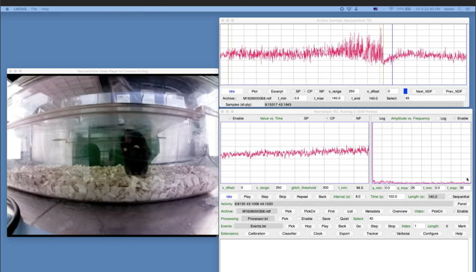
[06-JUN-25] Our transmitters provide one or more telemetry signals, depending upon how they are configured. We have two classes of telemetry receiver: coaxial antenna and antenna array. The coaxial antenna systems use antennas on the end of coaxial cables. We distribute the antennas among our Faraday enclosures, placing them between and adjacent to our animal cages. A coaxial antenna system will record from a hundred transmitters. Our Telemetry Control Box (TCB) is a coaxial antenna system. It provides an approximate animal location measurement for multi-room habitats, by reporting which of its antennas is receiving the most power from each telemetry channel. Our antenna array systems provide a platform upon which we can place one or two animal cages. Beneath the platform is an array of antenna coils. The array provides activity measurement in units of centimeters moved per unit time, and reliable disambiguation of animals in video recordings. Our Animal Location Tracker (ALT) is an antenna array.
| Assembly | Name | Type | Description |
|---|---|---|---|
| A3042A-16 | Telemetry Control Box (TCB) | Coaxial Antenna | 16 coaxial antennas, telemetry reception, location monitoring, PoE. |
| A3042B-16 | Telemetry Control Box (TCB) | Coaxial Antenna | 16 coaxial antennas, telemetry reception, command transmission, location monitoring, PoE. |
| A3038 | Animal Location Tracker (ALT) | Antenna Array | 15 coil antennas in 48 cm × 24 cm array, location tracking, PoE. |
| A3018 | Data Receiver | Coaxial Antenna | 1 coaxial antenna, telemetry reception, requires LWDAQ Driver. Discontinued 2016. |
| A3027 | Octal Data Receiver (ODR) | Coaxial Antenna | 8 coaxial antennas, telemetry reception, requires LWDAQ Driver. Discontinued 2022. |
| A3071 | LWDAQ Driver | TCPIP Interface | Required by all existing A3018 and A3027 receivers. |
The (A3042) Telemetry Control Box (TCB) and A3038 Animal Location Tracker (ALT) require only one Power over Ethernet (PoE) connection for power and communication combined. The A3042A-16 TCB provides sixteen antenna inputs, each with its own independent telemetry receiver. The A3042B-16 TCB provides the same sixteen antennas, but each antenna both receives telemetry signals and transmits commands to our radio-controlled devices. The ALT permits recording from all animals moving over its antenna array. The A3038C platform is 51 cm × 27 cm, so we can place one large rat cage or two small mouse cages upon a single platform.
| Assembly Number and Manual Link |
Assembly Name | Status |
|---|---|---|
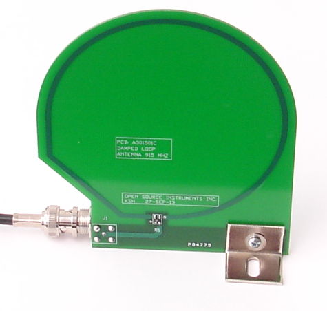
| A3015C | Damped Loop Antenna | Active |
| A3015E | Damped Loop Antenna | Active |
| A3039E | Coaxial Feedthrough | Active |
| A3039F | Ethernet Feedthrough | Active |
| FE3A | Bench-Top Faraday Enclosure | Discontinued |
| FE3B | Bench-Top Faraday Enclosure | Active |
| FE5A | Canopy Faraday Enclosure | Active |
| A2071E | LWDAQ Driver | Active |
| CEC-1 | Coaxial Extension Cable, 0.91 m | Active |
| CEC-2 | Coaxial Extension Cable, 2.3 m | Active |
| CEC-5 | Coaxial Extension Cable, 4.6 m | Active |
| CEC-8 | Coaxial Extension Cable, 7.6 m | Active |
| CEC-15 | Coaxial Extension Cable, 15 m | Active |
| HHS-1 | Hand-Held Spectrometer | Active |
A single A3042 Telemetry Control Box (TCB) provides sixteen antenna sockets on the back wall. Our older A3027 Octal Data Receiver (ODR) provides eight sockets. We connect these sockets to telemetry antennas with coaxial cables. The connectors are BNC connectors and the cables are 50-Ω high-frequency coaxial cables. We ship our antennas with 2.3-m cables. We include four short cables with each bench-top Faraday enclosure. The short cables connect antennas to BNC feedthroughs on the back wall of the Faraday enclosure. From the back wall to the telemetry receiver we use another cable, typically the 2.3-m cable. But if we want to place our telemetry receiver in a central location and run cables to our surgery station, behavior station, Faraday enclosures, and Faraday canopies, we can do so with the help of Coaxial Extension Cables, as listed in the table above. Each extension cable comes with a BNC union so you can join it to another cable. We see no significant degradation in telemetry reception with cables up to twenty meters long.
Our A3027 Octal Data Receiver is now discontinued, but many remain in operation, and we have no plans to discontinue support for them. They operate with a LWDAQ Driver. The ODR comes in a 30 cm × 22 cm × 11 cm metal box. The box connects to the LWDAQ Driver with a shielded network cable. It receives power through the same cable. Eight BNC sockets on the back of the box provide connections for a coaxial cables to the antennas. There are thirty indicator lights on the front of the box. There is one white light for each transmitter channel, one white light for each antenna input, and power, reset, upload, and empty lights. The Octal Data Receiver comes with eight Dampled Loop Antenna (A3015C). These attach to the antenna inputs with coaxial cables that pass through a Faraday enclosure wall with the help of a BNC feedthrough. Each antenna can stand on its own, or we can take the mounting brackets off and lay it on a table or wedge it between the cages in an IVC rack.
Here is a list of the families of telemetry sensors and radio-controlled implants we manufacture at OSI today, as well as families we have manufactured in the past, but have now discontinued in favor of the newer families.
| Assembly Number and Manual Link | Assembly Name | Status |
|---|---|---|
| A3028 | Subcutaneous Transmitter | Discontinued |
| A3048 | Subcutaneous Transmitter, One Input | Active |
| A3049 | Subcutaneous Transmitter, Two Inputs | Active |
| A3047 | Subcutaneous Transmitter, Four Inputs with Temperature | Active |
| A3040 | Head-Mounting Transmitter, Four Inputs | Active |
| A3041 | Implantable Stimulator-Transponder | Active |
| A3035 | Implantable Inertial Sensor | Active |
| A3051 | Blood Pressure Monitor | Planned |
Faraday enclosures can be bench-top with hinged doors, or they can be canopies supported by an aluminum frame around a free-standing rack of shelves. The bench-top enclosures have back walls made of aluminum sheet where we place coaxial and Ethernet feedthroughs to carry coaxial and Ethernet connections. The canopies have floors made of aluminum sheet to which we attach coaxial and Ethernet feedthroughs.
[19-JUN-25] Before investing in one of our telemetry systems, we suggest you send us your animal laboratory's latitude and longitude so we can consult the global mobile phone base station database for transmitters near your facility. Mobile phone networks that use the 902-928 MHz band are less common now than they were ten years ago, but they still exist. If you have one on the building opposite you, directing power right through your windows, your telemetry system will not perform well.
We recommend you set up your telemetry system several weeks before you plan to perform your first animal experiments. During these weeks, you can install our software on your computer and learn how to acquire and analyze telemetry signals. We supply one or two diagnostic transmitters with your telemetry system. These are not for implantation. Place your diagnostic transmitters within your telemetry system and record their signals continuously for a week to make sure that reception of telemetry signals is robust and that downloading and recording is continuous and reliable. Recording might be interrupted every few hours by scheduled activity on your computer or network. Reception may be interrupted at certain times of the day by an intermittent source of microwave interference. You will be glad to have solved such problems before you begin working with telemetry devices implanted in live animals.
We begin with three lists of equipment, one for a system with a Telemetry Control Box (TCB), one for a system with Animal Location Trackers (ALTs), and one for a system with a LWDAQ Driver and Data Receiver or Octal Data Receiver. In each list, we include Faraday enclosures. Most likely you will need these to isolate your telemetry system from local microwave interference, but if we have agreed to supply you with a telemetry system without Faraday enclosures, skip over the enclosure items in the list. Faraday enclosures for coaxial antenna systems come in two types: those for benchtop laboratory systems and those for use with shelf rack systems. We will mention both benchtop and shelf systems in our lists. When we say "network cable" we mean a "Cat-5 or Cat-6 Ethernet jumper cable". These can be shielded or unshielded. In our lists, we state which cables must be shielded. We begin with the list of parts required for a coaxial antenna telemetry provided by a TCB:
List of parts required for antenna array telemetry provided by Animal Location Trackers (ALTs):
List of parts required for coaxial antenna telemetry provided by a Data Receiver or Octal Data Receiver :
Assuming you have the above parts in hand, follow the set-up steps in the following paragraphs. These steps will take you through the organisation and configuration of your hardware and software. They show you how to test that your system is working well. By the end, you will be able to record from any of our telemetry sensors.
Connect AC Power: We provide a universal, 100-240V, 50-60Hz power adaptor for use with your telemetry system. If we shipped your system to you in the USA, we will ship a power cord along with your power adaptor. But if we shipped your system to you outside the USA, we will not attempt to ship you a power cord that fits your local power sockets. We will leave it to you to find a standard computer power cord for use with the power adaptor. If your telemetry system includes Animal Location Trackers (ALTs) or a Telemetry Control Box (TCB), we should have received a Power over Ethernet (PoE) switch along with your telemetry system. Connect your power cord to the PoE power adaptor and plug the power adaptor into the PoE switch. A green power light should illuminate on the PoE switch. If your telemetry system includes a Data Receiver (A3018) or Octal Data Receiver (A3027), you will also have in your telemetry system a LWDAQ Driver (A2071E or A2037E). Plug power into the adaptor that comes with the LWDAQ Driver, and plug this adaptor into the power jack on the back of the driver. The LWDAQ Driver power jack is on the back wall, next to the Ethernet socket. With power connected, green power lights should illuminate on the front side of the LWDAQ Driver.
Connect DC Power: If you have Faraday enclosures and ALTs, place your ALTs in your Faraday enclosures. We should have shipped you short and long ethernet cables with your ALTs. Connect each ALT to one an Ethernet feedthrough on the back wall of the Faraday enclosure. Use a short, shielded network cable to make this connection. Connect the feedthrough to the Power over Ethernet (PoE) switch. Use a long network cable to make this connection. This cable can be shielded or unshielded. White lights should flash once on the ALT when you connect it to the PoE switch. Green lights will remain illuminated. If you have a TCB, use a network cable to connect the Ethernet socket on its back wall to your PoE switch. This cable can be shielded or unshielded. Green lights should illuminate on the front panel of the TCB. If you have a Data Receiver(A3018) or Octal Data Receiver (A3027), connect it to the LWDAQ Driver with a shielded network cable. One green light should illuminate on a Data Receiver (A3018). Several green lights should illuminate on an Octal Data Receiver (A3027). Make a note of which socket on the LWDAQ Driver you have chosen for this connection. We recommend socket number one, which is the one closest to the LWDAQ Driver's indicator lamps, because that's the default socket number in the telemetry recording software you will be using in the steps below.
Connect Telemetry System to Data Acquisition Computer: If your telemetry system uses a Power over Ethernet (PoE) switch, connect your computer to the PoE switch with a network cable. This cable can be shielded or unshielded. Your computer must provide a wired Ethernet interface in order to make this connection. If your telemetry system uses a LWDAQ Driver connect the LWDAQ Driver and the computer directly with a network cable. Plug one end of the cable into the Ethernet socket on the LWDAQ Driver. Plug the other end into the computer's Ethernet socket. The Ethernet socket on the LWDAQ Driver is the RJ-45 socket on the back wall, next to the power jack. This network cable can be shielded or unshielded. Download the LWDAQ Software from the LWDAQ download page, or clone the LWDAQ GitHub repository. Go to the Software Installation chapter of our LWDAQ Manual and follow the software installation instructions for your operating system. Go to the Configurator chapter of the LWDAQ Manual and follow the instructions for establishing communication between your computer and your telemetry system. You will be setting up your computer and telemetry system on an isolated local network. You will need to know the IP address of your ALT, TCB, or LWDAQ Driver. The instruments all allow us to change their IP addresses, but when we ship them to you, they have an IP address that is easy to predict. All LWDAQ Drivers will have IP address 10.0.0.37. All ALTs and TCBs will have an IP address 10.0.0.X, where X is the last three digits of the instrument's serial number. If this number has a leading zero, drop the leading zero. The TCB with serial number Y71112 ships with IP address 10.0.0.112. The ALT with serial number P3012 has IP address 10.0.0.12. The first time you try to set up the Ethernet communication you are likely to find it difficult. But you only have to do it once for each computer, and the next time you have to set up a computer, it will go quicker. Once you can press the Contact button in the Configurator Tool and see a print-out of your telemetry system's version numbers and MAC address, you have succeeded.
Connect Telemetry System to Local Area Network (Optional): Once you have established communication between your computer and telemetry system, you may wish to configure the telemetry system to operate on your Local Area Network (LAN). Follow the instructions in the Configurator chapter of the LWDAQ Manual. You may have to work with your network administrator to obtain a "static IP address" for your telemetry system. The telemetry system does not support the dynamic host configuration protocol (DHCP). Your network administrator may not be happy about allowing you to put a strange device like an ALT, TCB, or LWDAQ Driver on their network. You must obtain permission from them to allow connections to "port 90" on the telemetry system.
For LWDAQ Drivers Only: Test Control of LWDAQ Power Supplies: If your receiver uses a LWDAQ Driver, you can test communication between your computer and the LWDAQ Driver at any time with the Diagnostic Instrument. Try turning on and off the LWDAQ power supplies and obtaining plots of the power supply voltages. When you turn off the power supplies, you will see the three power supply lights turn off.
Check Communication with Receiver: Open the Receiver in the LWDAQ Instrument Menu. Specify the internet protocol (IP) address of your receiver. If you are using a LWDAQ Driver, specify the socket on the driver into which you have plugged your receiver in the daq_driver_socket entry box. These sockets are numbered one to eight, with number one closest to the indicator lamps. Press Reset and Configure. You should see the red EMPTY light on the receiver flash briefly and then the Receiver Instrument will report your receiver type and firmware version number. Press Loop and you will see telemetry the Receiver downloading clock messages from your data receiver. Leave the Receiver Instrument looping. If it encounters an error, it will print out the error and stop. We don't want any such error to occur ever, so do not ignore these errors. We need to stop them from happening. If you cannot stop such errors from occurring, contact us by e-mail.
Coaxial Antenna Systems Only: Connect One Antenna: Connect a long coaxial cable to one of the antenna sockets on the receiver. Whenever you connect a BNC plug to a BNC socket, make sure that you turn the locking flange on the plug until it locks. If you don't lock the connector, your system will still work, but it will work intermittently, which makes it difficult to diagnose problems. Plug the other end of your long coaxial cable into a Telemetry Antenna (A3015).
Turn On a Diagnostic Transmitter: We provide two diagnostic transmitters with each telemetry system. Take one of these and place it near your coaxial antenna or upon one of your ALTs. If it's off, bring your magnet close to the transmitter and move it away again. A lamp should illuminate on your data receiver. On the Octal Data Receiver, TCB, and ALT there are white activity lamps. One of these should turn on. On the Data Receiver a single green activity lamp should turn on, although this lamp will be labelled "Receive". If the no activity lamp turns on, try again with the magnet. The transmitter should turn on and off easily. Once you have an activity lamp illuminated, hold the transmitter in your hand and move it away from the antenna. Eventually, you should see the activity lamp flickering. The activity lamp indicates signal reception. When reception is robust, the intensity of the activity lamp is constant.
View Transmitter Signal: You will now see the telemetry signal in the Receiver Instrument you opened earlier. Move your transmitter around with the leads dangling. The signal should be large and chaotic. Drop your transmitter in a beaker of water. The signal should settle down to the transmitter's input noise level. Set your transmitter down on the antenna, or beside the antenna. You should see 50 Hz or 60 Hz mains hum, depending upon your local AC power frequency.
Test Reception: Place a diagnostic transmitter near the antenna or antenna array. In the Receiver Instrument, you will see a status line below the signal display. This line tells you how many messages are being received from each active channel during each recording interval. By default, the recording interval is 1 s. With an active A3049E3, you should see 512 SPS (samples per second) from the transmitter. Move the transmitter around. If the activity lamp starts flickering, you will see the number of messages being received per second drop soon after in the Receiver Instrument's status line. Set the diagnostic transmitter down on your benchtop or on your ALT platform. If your ALT is inside a Faraday enclosure, leave the door open. Does reception drop every now and then? If so, you have an intermittent source of microwave interference. It could be a mobile phone, a cordless phone, a pager, or a microwave communication beam passing through your laboratory.
Coaxial Antenna Systems Only, Connect Additional Antennas: The Telemetry Control Box (TCB) has sixteen independent antenna inputs. The Octal Data Receiver has eight. Connect each antenna input to the back wall of a Faraday enclosure or to a Coaxial Feedthrough (A3039E) on the floor of your Faraday canopy. The bottom edge of the canopy curtain should fall between the line of BNC connectors on the feedthrough, and the feedthrough should be taped to the edge of the aluminum sheet floor of the canopy. On the inside of a Faraday enclosure, use a short coaxial cables to connect four antennas to the back wall feedthroughs. Inside a Faraday canopy, use long coaxial cables to connect eight antennas to the coaxial feedthrough. Distribute these eight antennas between your animal cages. If you find that you want to connect sixteen antennas to an Octal Data Receiver, this is indeed possible. You can connect two antennas to each of Octal Data Receiver input with the help of BNC T-adaptors. Make sure the antennas that share an input socket are separated by at least 30 cm and are at least 5 cm from the conducting walls of the enclosure. For an example of three antennas arranged adequately, see here. We recommend four antennas per Faraday enclosure, with none of the antennas in a single Faraday enclosure being combined with any other antenna in the same enclosure. We recommend eight independent antennas per Faraday canopy, or eight pairs of antennas with no antenna combined with any other antenna less than 60 cm distant. Test reception in your enclosures or canopy by moving your diagnostic transmitters from one place to another. Put them in a plastic cup containing 50 ml of water and repeat. If you get less than 95% reception anywhere in the enclosure, there is a problem with the system that needs to be fixed, so contact us by e-mail.
Record to Disk: Press Stop in your Receiver Instrument. Close the Receiver Instrument panel. In the Tool Menu, select the Neurorecorder. This Neurorecorder is a separate process from your original LWDAQ process. If you were to close the original LWDAQ process by pressing Quit, the Neurorecorder would keep running. In the Neurorecorder, enter the IP address of your TCB, ALT, or LWDAQ Driver. If you are using a Data Receiver or Octal Data Receiver, the driver_sckt needs to match the socket on the LWDAQ Driver into which you have plugged our Data Receiver or Octal Data Receiver. Press PicDir and select a directory into which you would like the Neurorecorder to write telemetry files. Choose a directory with no spaces in its path name. Do not choose "C:\EEG\Test Recordings", instead choose "C:\EEG\Test_Recordings". Press Start. The Neurorecorder will reset and synchronize the receiver. Once that is done, it will start recording to disk. There is no need for you to stop it. You can leave it running all the time. If you have ALTs, you must use a separate Neurorecorder for each ALT and a separate recording directory for the output files. Open more Neurorecorders using the Tool Menu in your original LWDAQ process and start them recording from your remaining ALTs.
Exercise the Neuroplayer: Select the Neuroplayer from the Tool menu of your original LWDAQ process. The Neuroplayer allows you to play signals you have recorded to disk, process those signals into summary measurements, and navigate through data archives to examine recorded signals. All these actions are explained in the Neuroplayer Manual. Select one of your live recording archives and press Play. Experiment with the frequency and voltage displays in the Neuroplayer.
Learn How to Perform Processing: Consult the Interval Processing chapter of the Neuroplayer Manual. This chapter contains several example processing scripts, including one that records telemetry reception efficiency to disk. Create a text file on your computer that contains processing instructions to record reception from your two diagnostic transmitters to a characteristics file on disk. We call them "characteristics files" because they record the characteristics of each interval of the recorded signals. In the Neuroplayer, use the Autofill button to fill in the channel select string by looking at what channels are present in your recording. Select your processor in the Neuroplayer and enable. With both transmitters set within your telemetry system, record their signals for several days. The signal playback and processing should proceed without interruption. The characteristics file recorded by the Neuroplayer will tell us how reception varies with time. These characteristics files are all text files with extension ".txt".
Learn How to Perform Analysis: Consult the Interval Analysis chapter of the Neuroplayer Manual. Download the Reception Averaging script and paste it into the Toolmaker. Read the comments in the code. Specify the channel numbers of your diagnostic transmitters. These might be single or dual-channel transmitters. Specify all the channel numbers they transmit. Set the averaging period to 3600 s. Press the Toolmaker's Execute button to run the script. A directory browser opens. Select the directory containing your characteristics files. The script will read all the characteristics files and print out the average reception per hour for the length of your recording. Plot reception versus time for your two diagnostic transmitters. The minimum performance we expect is reception greater than 80% for 95% of the time. In practice we see average reception of around 98%.
When our telemetry system consists of several receivers, we will need one Neurorecorder for each. If we want to process the signals as they are recorded, we will need at least one Neuroplayer per receiver. We may even need one Neuroplayer per animal. For example, we may have two animal location trackers (ALTs) with four animals over each tracker, and we want to export the signals from each animal to separate EDF files. We need two Neurorecorders and eight Neuroplayers. The Startup Manager allows us to define our telemetry recording and processing with a script and start all processes by running the script. After an interruption, we can re-start the system with a few mouse clicks.
[06-MAY-25] Reception of our telemetry signals is always limited by RF interference. Our faraday enclosures reduce ambient interference by a factor of one thousand. Where a single antenna receives the signal from an implanted transmitter 95% of the time, two independent antennas pick up the signal 99.5% of the time. Our Telemetry Control Box (TCB-A16) provides sixteen independent antenna inputs. Each input has its own amplifier, demodulator, and decoder. By distributing these antennas between our animal cages, the probability that at least one of them will receive any particular message approaches 100%. With eight antennas distributed through an IVC rack, for example, we obtained 100% reception everywhere within the rack, despite the presence of a 900-MHz mobile phone base station 80 m from the recording room. One TCB-A16 can record from dozens of animals in one such IVC rack. Our FE3A enclosure stands on its own, and is 90 cm wide, 60 cm high, and 65 cm deep. With a shelf half-way up, it holds six animal cages. With four antennas inside, it provides recording from forty cohabiting animals.
We define operating range as the greatest range from the pick-up antenna at which we obtain robust reception. An A3049B3 SCT transmits 512 messages per second, so the operating range is the greatest range at which we receive 410 or more messages per second in 95% of orientations and positions at the operating range. In practice, we operate the transmitters inside a Faraday enclosure, so their operating range must be adequate to cover the range from the antenna in the center of the enclosure to the farthest corner of the enclosure volume. For details of our studies of poor reception in various locations, see our Reception page.
Operating range without a Faraday enclosure varies dramatically with location. In Harwell, UK, in a rural location, we obtained robust reception out in the open at up to 200 cm. In a basement laboratory in Boston, operating range in the open was 150 cm. In a second-floor office in Waltham, MA, operating rante was 70 cm. In the tenth-floor animal room at ION in London, operating range with no enclosure is 20 cm. Decreasing operating range is the result of ambient interference. If you are operating in a basement or in a windowless, central room of a brick building, we suggest you first purchase a hand-held microwave spectrometer and measure your background interference. With this measurement, we can advise you on whether or not you need to include Faraday enclosures in your system.
In all other locations, we recommend you operate in Faraday enclosures, even though they are expensive and add a complication to your study. If your location is not protected by several meters of earth or brick, anyone can put a stop to your study at any time by starting up a 900-MHz GSM base station within a hundred meters of your location. So it's not worth taking the risk just to avoid the expense and inconvenience of the enclosures. We call them Faraday enclosures so we don't get them confused with animal cages, which are used to contain animals. Usually, these conducting cages are called Faraday cages. Our Faraday enclosures are all equipped with microwave absorbers inside, without which they do not function well at all. We describe the performance and construction of Faraday enclosures in Faraday Enclosures. Because Faraday enclosures give us at least a 20-dB (one hundred-fold) reduction in ambient interference, they increase the operating range of our transmitters by a factor of 10 (square root of one thousand). Even if the operating range is only 20 cm without a Faraday enclosure, it will be 200 cm within a Faraday enclosure.
[09-JAN-26] The sample throughput of our telemetry system is the number of unique samples it provides every second. If we have forty sensors, and each sensor transmits 512 SPS (samples per second), we would like the sample throughput to be 20,480 SPS. If you find that you are seeing warnings in your Neurorecorder about corrupted data, or warnings in the Neuroplayer about extra samples, or if you are seeing signal loss more than 5% in your recordings, it might be that the sample rate from all your sensors combined is exceeding the maximum sample throughput of your telemetry system. In this chapter we present the two factors that limit sample throughput in our telemetry systems. We provide rules for calculating the maximum sample throughput of any particular arrangement of Faraday enclosures, antennas, and telemetry sensors.
The first limit to sample throughput is the collisions that occur between sensors. A collision occurs when two sensors attempt to transmit a sample at the same time. Each sample is transmitted as a message. Each message contains eleven synchronizing bits, an eight-bit channel number, and a sixteen-bit sample value. It takes a sensor τ = 7.0 μs to transmit one message. In the appendix to this manual, we describe how our telemetry sensors use random scattering of transmissions to avoid systematic collisions. Here we assume that sensors collide at only at random. Consider a particular message transmitted by a particular sensor. Sensors do not collide with themselves, they collide only with other sensors. We do not need to know the sample rate of this particular sensor, we need to know only the total sample rate, R, of all the other sensors that share the same receiving antennas. If any one of these starts transmitting at any time from τ before our message begins until the moment the message ends, the two messages collide. Provided that 2Rτ << 1, almost all collisions will be between only two sensors, not three or more, and the probability of collision will be close to 2Rτ
At any particular antenna, when two messages collide, if the radio-frequency power received by the antenna from one sensor is ten times more powerful than the the power received from the other sensor, the more powerful message will be received and the weaker message will be lost, regardless of which one started first. But if neither is ten times more powerful than the other, the two messages corrupt one another and are both lost. As a telemetry sensor moves around and rotates, the radio-frequency power received by any particular antenna will vary by at least four orders of magnitude. Because of this dramatic variation, it is more likely than not that one of the messages will dominate the other. Let the probability of domination be ρ. The probability that any given message will be lost due to a collision is (1 − ρ) + ρ/2 = 1 − ρ/2. If ρ = 1.0, the probability of loss due to a collision will be at its minimum value of 50%. If we have n receiving antennas, the probability that any given message will be lost when it collides with another will be (1 − ρ/2)n. We would like ρ to be higher rather than lower, so that our loss from collisions is minimized. We increase ρ by placing our antennas nearby and distributing them evenly. In doing so, we make it more likely that there will be an antenna that is much closer to one of the colliding sensors than the other. All other things being equal, the power an antenna receives from a sensor drops by a factor of ten if it is three times farther away.
Combining our collision and loss probabilities together, we see that the probability that any particular message will be lost due to a collision is 2Rτ(1 − ρ/2)n, where R is the total sample rate of the other sensors, n is the number of antennas within range, and ρ is the probability that one colliding message dominates the other at any particular antenna. Let us say that the loss due to collisions should be no more than 5%. With this constraint, we obtain a maximum value for R, which we call the collision limit. There are only two cases of particular interest to us these days: four antennas in a benchtop Faraday enclosure or sixteen antennas in a free-standing Faraday canopy. In the table below, we present the maximum sample throughput for various numbers of antennas and for various values of ρ.
| Number of Antennas |
Domination Probability |
Maximum Colliding Sample Rate (SPS) |
Max 1-Channel 1024 SPS |
Maximum Throughput (kSPS) |
Example System |
|---|---|---|---|---|---|
| 1 | 1.0 | 7.1 | 8 | 8.2 | benchtop, animal location tracker |
| 4 | 0.6 | 14.9 | 16 | 16 | benchtop, antennas bunched up |
| 4 | 0.7 | 20.0 | 21 | 21 | benchtop, antennas on floor |
| 4 | 0.8 | 27.6 | 28 | 29 | benchtop, antennas on shelf and floor |
| 8 | 0.6 | 62.0 | 62 | 63 | canopy, antennas bunched up |
| 8 | 0.7 | 112.1 | 110 | 110 | canopy, antennas spread out |
| 8 | 0.8 | 212.6 | 210 | 210 | canopy, antennas among cages |
| 16 | 0.6 | 1074.7 | 1000 | 1100 | canopy, antennas bunched up |
| 16 | 0.7 | 3517.5 | 3400 | 3500 | canopy, antennas spread out |
| 16 | 0.8 | 12659.7 | 12000 | 13000 | canopy, antennas among cages |
To estimate the value of ρ, we placed ten A3049Q4 SCTs in our own FE5B Faraday canopy. Together, these transmitters produced 20 kSPS, which is perfect for observing collisions. We equipped the canopy with four antennas, which we placed at the four corners of a table. We arranged the ten transmitters on the table and measured average signal loss. We re-arranged the transmitters and measured average signal loss again. In all arrangements and for all SCTs, the average loss was around 5%. When we added four more antennas and loss dropped to 1%. When we tried four antennas with only two of the SCTs running, average loss was less than 1%. These observations are consistent with our loss being dominated by collisions, and with ρ = 70%.
The second limit to sample throughput is the data receiver itself. We call this the receiver limit. Each receiver limits sample throughput in its own way. The receiver limit of an Animal Location Tracker (ALT) arises from the speed with which it can read out its detector modules, which is 45 kSPS. But an ALT acts as a telemetry system with one antenna and collision domination probability 100%, which fixes its collision limit at 8.2 kSPS. The collision limit is far below the receiver limit, so the ALT's sample throughput is limited by collisions, not by the ALT itself. The receiver limit of a Telemetry Control Box (TCB) with the latest firmware is 320 kSPS. When a TCB with sixteen antennas receives the same sample on all sixteen antennas, it has to read out and examine all sixteen copies of the sample. If all sixteen antennas receive sixteen copies of every sample, the maximum sample throughput is 320 kSPS / 16 = 20 kSPS. The collision limit for this same arrangement >1000 kSPS, so the maximum throughput of a TCB with sixteen antennas in one enclosure is limited by the TCB itself, not by collisions. If we connect the TCB to four enclosure, each with four antennas, we will receive only four copies of each sample, so our receiver limit will be 320 kSPS / 4 = 80 kSPS. The collision limit for each of these enclosures is roughly 20 kSPS as well, making 80 kSPS for the four of them together, so in this arrangement, the collision and receiver limits are approximately the same. The receiver limit of our Octal Data Receivers (ODR, A3027) is imposed by the size of its message buffer. The ODR message buffer is 512 KByte and each ODR message is 4 bytes. In order to maintain reliable data acquisition from an ODR, we would like its message buffer to hold two seconds of telemetry date. The buffer will hold 512 KByte / 4 bytes per message = 131072 messages. If the buffer is to hold two seconds of telemetry data, the telemetry throughput is limited to 65535 messages/second. As a rule of thumb, we assume the receiver limit for the ODR is around 64 kSPS.
To increase the maximum sample throughput of our telemetry system, we arrange our antennas so that they are close to our animal cages and uniformly distributed among them. This increases the probability that when two sensors collide, each will be much closer to one of the antennas than the other, which in turn increases the probability that both messages will be received: one by its nearby antenna and the other by its own nearby antenna. In some systemns, it is the receiver itself that limits the maximum sample throughput. Our TCBs will impose a limit our throughput if we deploy all sixteen antennas in an environment where every sample is received by every antenna. Fewer antennas in each Faraday enclosure will maximize TCB throughput, but at the same time, fewer antennas increases loss due to collisions and loss due to interference. If you see data corruption errors extra sample warnings, or poor reception, consider increasing or decreasing the number of antennas in your enclosures.
WARNING: Do not soak our implantable devices in ethanol for more than ten minutes.
[19-JUL-26] All our implantable devices, such as our Subcutaneous Transmitters (SCTs), Intraperitoneal Transmitters (IPTs), and Implantable Stimulator-Transponders (ISTs), are encapsulated in epoxy and coated with silicone. The first time you implant a particular device, you remove it from its bag and subject it some procecure that kills all microbes that might be living on the surface of the device. Some of our customers call this process sterilization. Others call it disinfection. So far as we know, they mean the same thing. After disinfection, you implant the device in its host animal and perform your experiment. When your recording is complete, you will either discard the animal and the device together, or you might remove the device from the host, hoping to use the device again in another host animal. We call this removal explantation. Explantation is worth doing only if the device has sufficient operating life remaining for a second experiment. Befor re-implanting the device, you must dissolve and wash away any residual dental cement around the device's electrodes, cut away remaining scar tissue from around the leads, and wash off hair and blood that adheres to the device's silicone coating. We call this process cleaning. The final stage of cleaning is to rinse the device in water and dry it off. Now you put it back in the package we provided, make sure it is turned off, and put it on a shelf. We say the implant is now in storage, awaiting re-implantation. We discuss disinfection, cleaning, and storage in separate paragraphs below. Our objective is to make sure your disinfection, cleaning, and storage are effective, but at the same time avoid causing damage to the implant or exhausting its battery.
We recommend four different ways to disinfect implantable devices: ethanol wash, ethylene oxide gas, boiling water, and autoclaving. To sterilize with ethanol, stirr or shake in ethanol for ten minutes. You may use 70%, 95%, or 100% ethanol at room temperature. In one of our experiments, soaking four implants in ethanol for one hour at room temperature caused no damage to any of the implants, but soaking for four hours damaged all four. In order to be certain that your ethanol sterilization causes no damage to your implants, we ask you to restrict the ethanol immersion to no longer than ten minutes. Sterilization with ethylene oxide gas subjects the device to 60°C and 80% humidity for six hours. This temperature causes no harm to the implant's battery and six hours is insufficient time for water vapor to cause corrosion even 60°C, so this gas sterilization is perfectly safe. Boiling water is often useful as a disinfectant because it can kill certain germs that are resistant to ethanol. To disinfect with boiling water, drop your implants into boiling water for ten minutes, but no longer. Ten minutes is not long enough for corrosion to start, but our calculations suggest that an hour will put the transmitter at risk. You may use an autoclave to disinfect your implants, provided you limit the temperature and duration of the autoclave process. Autoclave at 121°C and atmospheric pressure for no more than thirty minutes. Autoclave at 132°C and atmospheric pressure for no more than fifteen minutes.
Our devices are encapsulated in epoxy and coated with silicone. Acetic acid does not react with silicone or epoxy any more than does water. Acetic acid dissolves cured cyanoacrylate, so it can be useful for cleaning off cyanoacrylate used to fix electrodes in place during implantation. Feel free to soak our implants in acetic acid at room temperature for one or two days. Acetone dissolves dental cement and cyanoacrylate, so it will dissolve and remove the cement you use to construct head fixtures. Place your device with dental cement in acetone in a sealed jar at room temperature for six hours. Shake occasionally. Dispose of the dirty acetone. Rince the implant twice in clean acetone to remove all dissolved cement. Now rinse in water to remove the acetone residue, and dry off. By this point, the device should be clean. Do not leave your implant soaking in acetone for more than six hours. Acetone dissolves in silicone and reacts with epoxy, so prolonged exposure to acetone will damage the encapsulation. See Silicone and Solvents for further discussion of acetone as a cleaning fluid. Ethanol dissolves slowly with silicone and epoxy at room temperature. As we mention above, in our paragraph on disinfection, we ask that you refrain from soaking your implants in ethanol for more than ten minutes. When left to soak in ethanol, the silicone coating will begin to feel slimy to the touch. Eventually the silicone will swell and crack. The epoxy swells also, and when we subsequently implant an ethanol-damaged implant in an animal, the ethanol will evaporate from the epoxy, leaving cavities and cracks behind, as we show in our photographic report Degradation of Epoxy by Ethanol. These cavities will fill with condensed water vapor that comes into contact with the implant's electronic components, causing the implant to malfunction and drain its battery.
When you store an implant, store it in a dry place at room temperature. Do not store it in any kind of fluid, not even water, and certainly not acetone or ethanol. Assuming the device is dry, it will tolerate storage at any temperature −20°C to 60°C. Provided relative humidity is less than 80%, corrosion within the implant circuit will be slowed to a standstill. The more difficult component to proper storage is making sure the device stays off. Most of our implantable devices turn on with a magnet. Touch them with a magnet and they turn on. Touch them again and they turn off. When we store these, we must first make sure they are turned off, and then store them on a shelf far from any source of magnetic fields. The rest of our devices sleep when they are placed on a magnet. When we store these, we must make sure they stay sitting on the magnet in the storage box we used to ship them to you. Store all implants at least 30 cm from any electrical power supplies, magnets, or large lumps of iron.
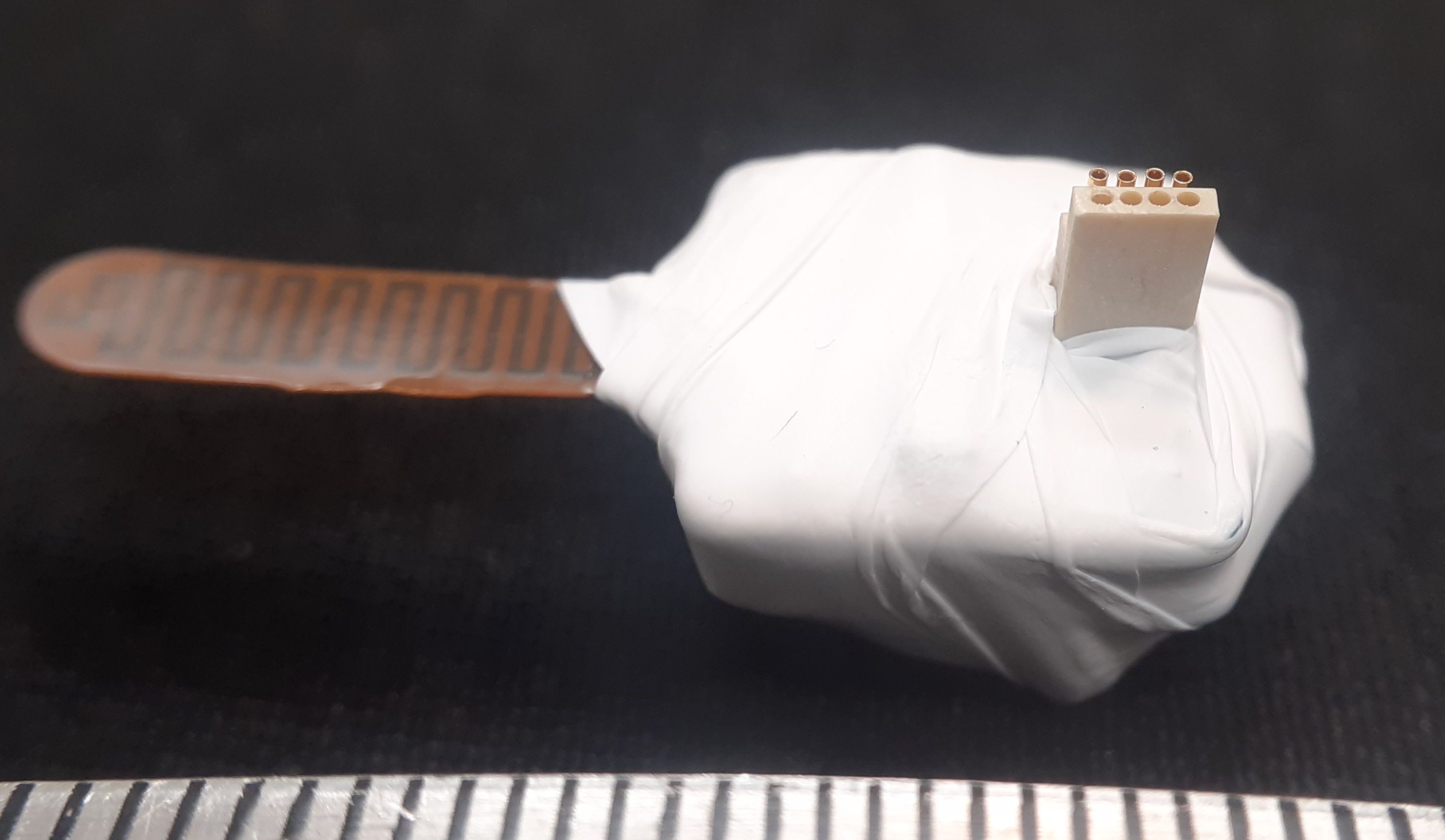
Our Head-Mounting Transmitters (HMT) are not implantable. Nor are they coated in silicone. The HMT is a bare circuit board into which you load a battery, fold up, wrap with teflon tape, and attach to the head of a host animal. It is never implanted. It does not have to operate while immersed in warm saline. Because the HMT is a bare circuit board, however, it is vulnerable to electrostatic discharge. Whenever you carry an HMT, carry it in the anti-static bag in which we shipped it to you. Do not carry an HMT in your bare hands while wearing rubber shoes. While sitting and handling the HMT out of its bag, cover static-generating clothes with a laboratory coat. You may disinfect your HMT using any of the processes we recommend for implantable devices in the preceding paragraphs. When you detach an HMT from a host animal, you unwrap its tape and remove the battery. Clean the HMT by washing it in warm running water and scrubbing gently with a toothbrush. After cleaning, dry with compressed air or dab with lint-free cloth and allow to dry in ambient air for twenty-four hours. Now store the HMT in its anti-static bag.
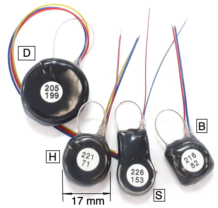
[06-JAN-26] Our existing telemetry sensors provided between one and four biopotential inputs. These might share a common reference potential, as in the two-channel A3049H2, or they might each have their own reference potentials, as in the four-channel A3047A3D-C. The figure below is an example of the frequency response we obtain during final quality control of a batch of transmitters before shipping.
In our telemetry sensor version tables, we describe each input by its sample rate, high-pass filter frequency, low-pass filter frequency, and input dynamic range. If the amplifier has no high-pass filter, we call it a "DC Transmitter". Otherwise we call it an "AC Transmitter". All SCTs and HMTs come in both AC and DC versions. The DC versions have a "Z" in their part number. The dynamic range of the AC transmitters is typically 30 mV, arranged as −18 mV to +12 mV. The dynamic range of DC transmitters is typically 120 mV, arranged as −72 mV to +48 mV. The larger dynamic range allows the DC input to accommodate the largest possible galvanic potential generated by its electrodes. All biopotentials are digitized to sixteen-bit precision before transmission. The raw telemetry signals we read from an NDF file are all sixteen-bit numbers. The value 0 cnt (zer counts) represents the bottom of the dynamic range. The number 65565 cnt represents the top of the dynamic range. We obtain the conversion factor from counts to voltage by dividing the dynamic range by 65536. For input with range 30 mV we use 0.46 μV/cnt, and for an input with range 120 mV we use 1.8 μV/cnt.
When we drop a transmitter in water, we see the electronic noise generated by the transmitter circuit added to the chemical noise generated by the electrodes as they react with the water. With only stainless steel wire for the electrodes, this chemical noise is negligible. For our standard amplifier with gain ×100 and input impedance 10 MΩ, electrical noise is around 5 μV rms in 1-160 Hz, referred to the analog input. With gain ×10 the electrical noise increases to around 10 μV rms in 1-160 Hz.
The distortion of a signal by our telemetry system is the extent to which it changes the shape of a signal. We apply a 10 mVpp sinusoid to the X and Y inputs of an A3049AV3. The AV3 is equipped with two 160-Hz amplifiers. Input dynamic range is 30 mV. We increase the frequency from 1/8 Hz to 200 Hz. For each frequency, we obtain the spectrum of the signal and measure the power outside the sinusoidal frequency as a fraction of the sinusoidal power using this script. We express the result in parts per million.
The distortion of the X is dominated by random electronic noise. There are no significant peaks in the spectrum outside the fundamenta.
Note that the distortion generated by the new A3047, A3048, and A3049 transmitters is hundreds of time less powerful than that of their predecessors (A3013, A3019, and A3028). The new transmitters sample their signals uniformly, thus eliminating the scatter noise present in earlier devices.
An artifact in one of our biopotential recordings is an unwanted addition to the potential that is generated by some process outside the telemetry sensor. The most common source of artifact is movement. The top four sources of movement artifact in iEEG recordings made with wireless telemetry sensors are as follows:
[09-FEB-24] Our telemetry system supports four types of activity monitoring. None of the measurements are perfect, but all are useful. The four types are: location monitoring, location tracking, acceleration recording, and acceleration with rotation recording. The first two are provided by the telemetry receiver. The second two are provided by a dedicated implant that holds an accelerometer and gyroscope: the Implantable Inertial Sensor (IIS).
The Telemetry Control Box (TCB) measures the radio-frequency power received by each its antennas whenever it receives and decodes a telemetry message. It provides to us the number of the antenna that received the greatest power and a logarithmic measurement of that power. We call these the top antenna and the top power. In a telemetry system in which the antennas are separated by at least thirty centimeters, the top antenna is almost certainly the one closest to the transmitter. Thus the TCB allows us to determine the location of an animal in a maze or some other environment with multiple chambers. We call this location monitoring.
The Animal Location Tracker (ALT) measures the radio-frequency power received by each of its detector coils whenever it receives and decodes a telemetry message. It provides us with a logarithmic measurement of this power at each of its coils. By taking a weighted centroid of the receive power, the ALT provides us with a location. This location is not an accurate measurement of the location of an animal, but its movement is well-correlated with the movement of the animal, and its value is well-correlated with position. We can use the centroid to obtain a measurement of total distance traveled by each animal in a cage. We can measure the time pairs of animals spend close together. We can use the movement of the centroid to determine which animal is which in continuous video recordings. We call this location tracking.
Both location monitoring and location tracking come at no cost in operating life of the transmitter. We can perform both measurements with any telemetry device that transmits telemetry messages. If we want a higher-resolution measurement of the acceleration of an animal, we must implant an accelerometer. We will obtain 64 SPS of acceleration measurements in three orthogonal directions. We call this measurement acceleration recording. The accelerometer-only versions of the IIS provide acceleration recording. If we want to measure acceleration and rotation, the accelerometer with gyroscope versions of the IIS provide acceleration with gyroscope recording. The gyroscope is power-hungry, so the IIS with gyroscope supports intermittent measurements over a long period, but not continuous measurements.
[30-NOV-21] We have a library of example telemetry recordings available on our Example Recordings page. You will also find two short example recordings in the LWDAQ/Images folder: they are the two files with extension "ndf".
For a tutorial on browsing recordings with the Neuroplayer, see our Neuroplayer Introduction video.
[12-JUL-23] Our telemetry system records its telemetry signals to disk in files that conform to our Neuroscience Data Format (NDF). An NDF file begins with the characters " ndf" followed by a four-byte metadata string address, a four-byte data address, and a four-byte metadata string length. The byte ordering is big-endian (most significant byte first). The telemetry data is in the data section, with one record saved per unique message received from the telemetry system. We describe the message format in detail elsewhere, but we will summarize the format here. Each message consists of a core and a payload. The core is four bytes long. The first byte is the telemetry channel identifier. The next two bytes are the message data value, which almost always be a sixteen-bit sample value with its most significant byte first. The fourth byte of the core is a timestamp. The payload consists of further bytes of information obtained from the telemetry receiver. Some receivers produce no payload. Others produce payloads up to sixteen bytes long.
| Receiver | Payload (Bytes) |
Description |
|---|---|---|
| A3018 | 0 | Data Receiver, no payload |
| A3027 | 0 | Octal Data Receiver, no payload |
| A3038 | 16 | Animal Location Tracker, sixteen detector coil powers |
| A3042 | 2 | Telemetry Control Box, top power and top antenna |
The program that does the recording is the Neurorecorder, which is a tool build into our LWDAQ software. The Neurorecorder writes "payload" field to the NDF metadata string, in which it notes the length of the message payload in the NDF file's messages. The Neurorecorder knows the payload length because it queries the receiver to determine the receiver version, and from this version number the Neurorecorder deduces the message payload length. Here is an example metadata string from an NDF recorded from an Animal Location Tracker (ALT).
When we play an NDF recording in the Neuroplayer, the Neuroplayer reads the payload length from the metadata and acts accordingly. The payload provided by an ALT contains the power of the message at each of the ALTs location and auxiliary detectors. The power bytes, combined with the spatial distribution of the ALT's detector coils, allows us to deduce the approximate location, and measure the activity of animals. The "alt" field in the metadata gives the locations of the detector coils in a three-dimensional coordinate system. The payload provided by the TCB gives us the maximum power with which the message was received by any of the TCB's detector coils, and the identifier of that detector coil. The "alt" field for a TCB recording would likewise provide us with the locations of the detector coils, and the top antenna will give us an idea of where the animal is in a large space, or a multi-room habitat, in which we have one or two antennas in each room.
[11-SEP-25] Our electrode leads are made of a flexible coil of stainless steel wire that we insulate with two coats of silicone. The surface coat is a clear, unrestricted, medical-grade silicone such as MED-6607. The core coating is a tough and elastic silicone such as SS-5001 to which we have added a dye to give the lead a bright color. Available lead colors are: blue, red, orange, purple, yellow, green, pink, and brown. See our Flexible Wires page for detailed discussion of the design, manufacture, and use of our flexible wires and antennas.
| Lead Code |
Outer Diameter (mm) |
Spring Diameter (μm) |
Wire Diameter (μm) |
Resistance (Ω/cm) | Mass (mg/cm) | Maximum Length (mm) |
Names |
|---|---|---|---|---|---|---|---|
| B | 0.7±0.1 | 450 | 100 | 6.3 | 10 | 280 | Thin Lead |
| C | 0.5±0.1 | 250 | 50 | 25 | 5 | 130 | Very Thin Lead |
| D | 0.8±0.1 | 500 | 150 | 1.6 | 13 | 130 | Stimulator Lead |
We can manufacture B-Leads up to 280 mm long and C-Leads up to 130 mm. The 0.5-mm diameter C-Leads leads are far more flexible than the 0.7-mm B-Leads leads. They are less likely to cause irritation and infection in the subject animal. But the spring in the C-Lead is delicate. Its wire is half the diameter of the wire in the B-Lead. The spring itself is one quarter as strong. They will survive the fatigue of animal movement, but they are easy to damage with a scalpel during implantation or extraction. Removing insulation from a 0.5-mm lead is a delicate operation. Furthermore, we cannot provide screw or pin terminations on 0.5-mm leads because the wire breaks so easily at the edge of the solder joint. We can, however, solder the 0.5-mm leads to X-Electrodes directly and insulate with silicone afterwards, which is what we do for electrode interface fixtures such as the EIF-XAAX.
The D-Lead we can manufacture up to 130 mm long. These leads have low resistance. We at some point thought they would be useful for delivering current to Implantable Light-Emitting Diodes (ILEDs). But our B-Leads proved sufficient for optogenetics experiments and we have never had any need to deploy D-Leads on SCTs.
Consult the Insulation Removal chapter of our Flexible Wires page for detailed instructions on how to remove insulation from our 0.5-mm and 0.7-mm leads. Consult the Solder Joints chapter for instructions on tinning stainless steel for soldering to screws and pins.
[31-OCT-25] We provide a variety of terminations for our electrode leads, and a variety of depth electrodes to which these terminations can be connected. See Electrodes and Terminations for a list of terminations and depth electrodes with links to photographs and drawings. For electrode implantation instructions see our Electrode Surgical Protocols.
[17-JUN-25] The table below lists the various antennas we use with our 915-MHz telemetry system. They vary in length, material, and shape. We will recommend an antenna based upon your animal mass, implant operating life, and implant type.
| Antenna Code |
Length (mm) |
Description |
|---|---|---|
| A | 50 | Stranded steel loop antenna, 360-μm diameter 7×7 304SS wire, insulated in clear MED-6607 silicone, for transmitters in rats. |
| B | 30 | Stranded steel loop antenna,
360-μm diameter 7×7 304SS wire, insulated in clear MED-6607 silicone, for transmitters in mice. |
| C | 13 | Straight antenna of coiled steel wire, 450-μm diameter 316SS coil. Discontinued. |
| D | 30 | Stranded steel loop antenna, 250-μm diameter 7×7 304SS wire, insulated in clear MED-6607 silicone, for transmitters in small mice. |
| E | 50 | Stranded steel loop antenna, 250-μm diameter 7×7 304SS wire, insulated in clear MED-6607 silicone, for radio-controlled implants. |
The 50-mm A and E antennas produce the strongest signal when implanted in rats. The 30-mm B and D antennas fit easily into mice without folding. The D and E antennas are made with a thinner stranded wire. We can fold the 30-mm D antenna through 45° with a 1-g force, while the 30-mm B antenna requires a 4-g force. Because of their flexibility, the D and E antennas are a natural choice for mice and rats respectively. The A and B antennas are, however, more resistant to fatigue. For implantations longer than three months, we recommend the A and B antennas. We no longer make the C-Antenna because it transmits ten times less power than the loop antennas, while the D-Antenna is just as easily accommodated by a small animal as the C-Antenna.
[24-SEP-25] Our standard implantable devices and all our head-mounting devices are powered by lithium primary coin cell batteries. These batteries provide the longest possible operating life per unit volume. In our implantable transmitters, the rigidity and hermetic seal of the coin cell makes it easy to encapsulate and resistant to corrosion. In our head-mounting devices, the convenient disk shape of the coin cell allows it to be mounted with a clip, so we can replace it easily. The output voltage of a lithium primary cell remains close to 3.0 V throughout their operating life.
Coin cells has steel cases, so they are magnetic. They are not suitable for deployment in strong magnetic fields. When an implantable device must operate within a magnetic resonance imaging machine, we equip it with a non-magnetic lithium-polymer battery and we disable its magnetic switch. The output voltage of a lithium-polymer battery starts at 4.2 V and drops to 3.5 V during the course of its life, as you can see here and as presented here. We do not make non-magnetic head-mounting devices because non-magnetic batteries do not come in coin cells.
Our Implantable Stimulator-Transponders (IST) provide an accurate and deliberate measurement of battery voltage that it provides whenever we communicate with it using the Stimulator Tool. Our Subcutaneous Transmitters (SCT) and Head-Mounting Transmitters (HMT) provide no deliberate measurement of battery voltages, but their AC-coupled versions do provide an incidental measurement of battery voltage through the average value of their signals. The average value of the AC-coupled SCT signal is a function only of the internal 1.8-V power supply voltage used by its amplifier. If the offset in the amplifier is zero, and the on-board 1.8-V voltage regulator produces exactly 1.80 V, the transmitter's battery voltage is given by following formula.
Where VB is the battery voltage and SA is the average value of the signal in sixteen-bit ADC counts (cnt). The value of SA lies in the range 0-65535. In practice, this formula is accurate to ±0.1 V so long as the battery voltage is ≥2.4 V. During the life of a typical SCT or HMT battery, its voltage will be close to 3.0 V, so we expect the average value of an AC-coupled signal to be close to 1.8 V * 65535 / 3.0 V = 39321. If the signal is DC-coupled and the average voltage applied to the input happens to be exactly 0 V, we will see the same 39 kcnt average signal value. The plot below shows how the average X and Y vary for an A3049A3 SCT as we decrease battery voltage from 3.4 V down to the minimum voltage at which the transmitter will continue to operate, which is 1.8 V.
As the battery voltage drops below 2.4 V, the average value of X drops towards zero, while the average value of Y continues to rise. We see similar behavior in the A3048 and A3047 families of SCTs, as well as the A3040 family of HMTs. An AC-coupled SCT's battery voltage measurement is reliable for 99% of its operating life, but once the battery is near exhausted, the measurement fails.
The average value of a DC-coupled SCT input is not so useful. Whatever long-term average value we record might be dominated by a galvanic potential on the input electrodes. Indeed: the purpose of DC-coupled transmitters is to record long-term galvanic potentials. Our existing Implantable Inertial Sensors (IIS) and Blood Pressure Monitors (A3051) provide no means to measure battery voltage.
[14-FEB-26] The battery life of Subcutaneous Transmitters (SCT) and Head-Mounting Transmitters (HMT) is a linear function of sample rate and battery capacity. The operating life of Implantable Stimulators (IST) is more difficult to estimate. On our IST page, you will find links to IST device family manuals, where you will in turn find operating life discussed in detail. The operating life of Implantable Inertial Sensors (IIS) is a strong function of the type of measurement it makes. Starting at our IIS page, go to an IIS device family manual and you will find battery life tabulated for the various types of measurement the family can perform. In the following paragraphs, we describe how the operating life of SCTs and HMTs can be deduced from their mass and sample rate.
The operating life of an SCT or HMT is how long it takes to consume its battery capacity in its active state. The shelf life is how long it takes to consume 10% of its battery while sitting on the shelf in its lowest-power state. To obtain the operating life of a device, we divide its battery capacity by its active current consumption. We wish to provide our customers with a specification of minimum operating life so they can plan their experiments with confidence.
Where Lo is the minimum operating life in days (d), C is the battery capacity in microamp-days (μA·d), La is the maximum active current consumption in microamps (μA), Iq is the quiescent current of the device (μA), α is the sampling current in microamp per sample per second (μA/SPS), and R is the total sample rate in sample per second (SPS). This total sample rate is the sum of the sample rates of all the device's inputs. If the transmitter has four inputs with sample rates 512, 256, 128, and 128 SPS, the total sample rate, R, is 1024 SPS. The following table gives maximum values for quiescent and sampling current so we can calculate the maximum active current for a particular total sample rate.
| Device Type |
Device Family |
Quiescent Current (μA) |
Sampling Current (μA/SPS) |
|---|---|---|---|
| HMT | A3040 | 25 | 0.12 |
| SCT | A3047 | 30 | 0.12 |
| SCT | A3048 | 18 | 0.12 |
| SCT | A3049 | 22 | 0.11 |
The heavier the battery, the greater its capacity. Manufacturers express battery capacity in mA·h (milliamp-hour). For our calculations, μA·d (microamp-day) is a more convenient unit. We have 1 mA·h (milliamp-hour) = 1000 μA·h (microamp-hour) = 42 μA·d (microamp-day). All our standard implantable devices and all our head-mounting devices are powered by lithium primary coin cells.
| Battery Type |
Battery Capacity (μA·d) |
Device Volume (ml) |
Device Mass (g) |
Comment |
|---|---|---|---|---|
| CR927 | 1250 | 0.85 | 1.5 | Smallest, often out of stock. |
| CR1216 | 1250 | 1.0 | 1.7 | Small, always in stock. |
| CR1225 | 2000 | 1.2 | 2.0 | Standard for mice. |
| CR1620 | 3300 | 1.4 | 2.9 | Standard for large mice. |
| CR2025 | 6700 | 2.1 | 4.8 | For juvenile rates. |
| CR2330 | 11000 | 2.6 | 6.0 | Standard for adult rats. |
| CR2450 | 25000 | 4.0 | 8.7 | Good for large rats. |
| CR2477 | 42000 | 6.0 | 14 | Only for largest rats. |
In order to record the shape and amplitude of a signal with frequency f Hz, our SCTs and HMTs must sample at 3.2f SPS. If we need only the amplitude of the signal, we can sample at a far lower rate, but almost all our SCT and HMT models sample at 3.2f in order to obtain a high-fidelity recording of the original signal throughout the input passband. For our SCTs and HMTs, the effective bandwidth of the input for the sampling process is the top frequency of the input passband. If the input passband is 2-80 Hz, we take the bandwidth to 80 Hz. To obtain the sample total sample rate of an SCT or HMT, we multiply the bandwidth of each input by 3.2 SPS/Hz to obtain the individual input channel sample rates, and add these together.
| Bandwidth (Hz) | Sample Rate (SPS) |
|---|---|
| 20 | 64 |
| 40 | 128 |
| 80 | 256 |
| 160 | 512 |
| 320 | 1024 |
| 640 | 2048 |
To obtain the total sample rate, R, of an SCT or HMT, we add the sample rates of all channels together. If, for example, we have four channels with bandwidth 160, 80, 40, and 40 Hz, the sample rates will be 512, 256, 128, and 128 SPS respectively. The total sample rate will be 1024 SPS. A dual-channel transmitter that provides 80-Hz bandwidth on both channels will have sample rate 256 SPS for each channel, and total sample rate 512 SPS.
To obtain the shelf life of an implantable device, we need to know its sleep-state current. When we turn off an SCT or IIS, it enters its sleep state. When we place an IST in its storage box, we place it on a magnet built into the box. This magnet causes the IST to enter its sleep state. Whe we remove an HMT's battery, it turns off completely. The table below give the maximum sleep currents for implantable and head-mounting devices.
| Device | Sleep Current (μA) |
|---|---|
| SCT (A3047, A3048, A3049) | 1.0 |
| HMT (A3040) | 0.0 |
| IST (A3041) | 2.0 |
| IIS (A3035) | 1.0 |
Our standard SCTs, IISs, and ISTs are all ferro-magnetic. Their coin cells are constructed out of steel casings. But we can manufacture non-magnetic versions of the same devices by equipping them with specialized, non-magnetic, lithium-polymer (LiPo) battery packs. These LiPo packs have lower capacity per unit unit volume than our lithium coin cells, but they contain no ferro-magnetic material. Our non-magnetic implants may be deployed in magnetic resonance imaging (MRI) machines. The table below gives the battery capacity of two LiPo packs suitable for non-magnetic implantable devices. Note that we are unable to provide a non-magnetic version of the HMT, because the HMT requires a coin cell battery.
| Battery Type |
Battery Capacity (μA·d) |
Device Volume (ml) |
Device Mass (g) |
Comment |
|---|---|---|---|---|
| GM-NM361215 | 1600 | 1.5 | 3.1 | non-magnetic for large mice |
| PGEB-NM651825 | 10000 | 4.5 | 8.7 | non-magnetic for adult rats |
In order to avoid being turned on an off while being moved in and out of a magnetic field, our non-magnetic implantable devices have their magnetic switches disabled. Non-magnetic SCTs and IISs run continuously from the moment we load their battery prior to encapsulation. Non-magnetic ISTs will be awake from the moment we load their batteries. The shelf life of a non-magnetic SCT or IIS is 10% of its operating life it is always active. You must implant them without delay to take advantage of their full operating life. Our non-magnetic ISTs do not sleep when stored on a magnet on the shelf. They are always awake. An A3041-family IST consumes 5.5 μA when awake, so its shelf life is 10% of C/Is.
None of our implantable devices are rechargeable. We experimented with rechargeable implants for several years and found them to be unreliable, toxic, and vulnerable to corrosion. They are unreliable because we cannot guarantee that our customers will connect the charging circuit correctly, nor that they will check the state of the battery before re-implantation. They are toxic because they emit gases when they are deeply discharged at the end of an experiment. They are vulnerable to corrosion because the battery expands and contracts as it is charged and discharged, creating cavities in which water can condense. Our collaborators lost too many animals to unresponsive rechargeable sensors and stimulators. Furthermore, rechargeable cells provide only half the capacity per unit volume of non-rechargeable cells, so the range of experiments we can perform with rechargeable cells is severely curtailed. Nor can the batteries in our implants be replaced. We offer no refurbishment program for implantable devices. We sell only brand new devices. You can implant them over and over again in different animals until their battery runs out, but once their battery runs out, their recording days are over.
None of our implants can receive power wirelessly. Wireless power delivery to imlantable devices is a popular idea, with many examples of groups and companies manufacturing such devices. Wireless charging works by generating an alternating magnetic field throughout the animal cage. The frequency of alternation varies from one design to the next: we have seen anything from 30 MHz to 915 MHz. If this alternating magnetic field passes through the power-harvesting coil on the implant, the field induces an electromotive force that the implant can use to charge a supercapacitor and power its operations. There are two serious problems with implants that obtain their power in this manner.
The first problem with wireless charging of implantable devices is that it is impossible to record high-fidelity biopotentials with metallic electrodes in the presence of an alternating magnetic field. Saline-metal junctions are non-linear and asymmetric (see Electrode Impedance). They act like crystal diodes, rectifying all alternating electromagnetic fields and generating a voltage that varies as the animal moves around in its cage. When we emit a 10-ms, 1-W burst of 150-MHz power into one of our own Faraday enclosures, we see 100-ms, 1-mV artifact in the iEEG of implanted transmitters. Wireless charging systems apply at least 1 W to their charging coils, so we expect to see an undulating 1-mV artifact in any signal recorded by metallic electrodes in a charging field, with pulses being adde when the animal moves violently, as it might in the event of an epileptic seizure.
The second problem with wireless charging is that it is unreliable. Power is harvested from the ambient charging field only when the harvesting coil is not parallel to the field lines. As soon as the coil stops with its plane parallel to the field lines, no power is delivered. It is only a matter of time before the implant supercapacitor runs out of power. Our continuous recordings are no longer continuous. If some of our test animals have a habit of resting in a particular corner of the cage where power harvesting fails, we will have signal loss that is correlated with behavior, and our study will be compromised. It is, in principle, possible to make a three-dimensional power harvester that picks one of two coils to harvest power, but there are further problems with this design, not the least of which is its increased implantation volume.
[03-SEP-25] Faraday enclosures ensure robust reception from implanted transmitters. They also make sure that the telemetry system conforms to all local radio frequency regulations, because the enclosure keeps our telemetry signals contained within its walls. We describe the development of our enclosures in Faraday Enclosures. A single FE3A benchtop enclosure, with a transparent shelf installed, accommodates six animal cages and provide recording from at least forty cohabiting animals. A single FE5A canopy enclosure accommodates an entire rack of eighty individually-ventilated cages. Not only is radio-frequency interference kept out of the enclosure, but so is low-frequency electrical noise such as mains hum. Conversely, the transmitter signals are confined within the enclosure. The signal power outside the enclosure is too weak for detection by standard instruments, which guarantees that the system violates no local radio-frequency transmission rules. Furthermore, we can operate multiple telemetry systems in the same room, because their signals will not interfere with one another.
[06-JAN-26] We may want to isolate our animals from sounds generated outside our telemetry system. According to our measurements, the steel mesh walls of our faraday enclosures do not provide any significant attenuation of sound in the range 200 Hz to 40 kHz. Clear vinyl sheet, however, is an excellent absorber of the ultrasonic frequencies audible to rats and mice. A curtain of overlapping vertical strips of vinyl provides a factor of one hundred reduction in the power of ultrasonic waves, while at the same time allowing ventilation.
Acknowledgement: We thank our customers for their help developing surgery protocols and describing the principles of surgery. We do not mention their names out of respect for their privacy.
[31-OCT-25] In the paragraphs bewlow, we make general comments about device implantation. You will find step-by-step instructions for implanting Head-Mounting Transmitters (HMTs) and Subcutaneous Transmitters (SCTs) in our Surgical Protocols page.
Adult mice tolerate single implants up to 15% of their own mass, or 3 g, whichever is less. Adult rats tolerate single implants up to 10% of their own mass, or 15 g, whichever is less. Juvenile mice and rats grow quickly, so the fractional mass of the implant decreases significantly within the a few days. Juvenile mice can tolerate an implant of 20% their mass, while rat pups can tolerate an implant of 15% of their mass. Both the volume and the mass of the implant are important, but our telemetry implants have density close to 2 g/ml (gram per milliliter), so we will talk only of the mass the implants. Given the same mass, however, a slim profile is better tolerated than a thick profile. The slim profile permits us to use a single-incision surgery protocol in mice, which causes them less trauma and accelerates their recovery. The slim profile distributes the implant mass over a wide area, reducing the stress on the tissue that holds the implant in place. If the thick and slim versions of the same transmitter were of equal mass, the slim version would always be the best choice. In practice, some of our slim versions are slightly heavier than our thick versions.
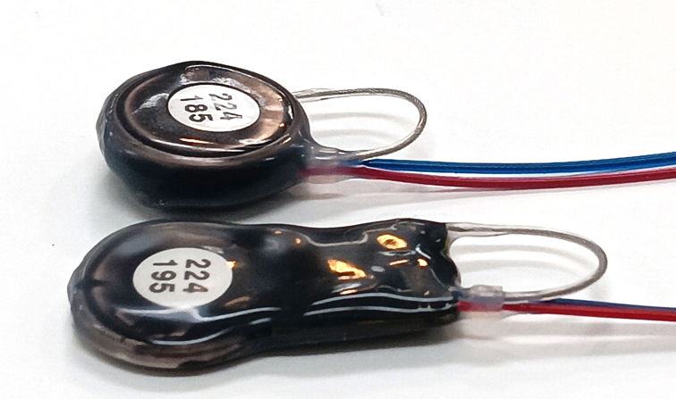
Most strains mice reach a mass of 10 g after 3 weeks and 20 g after 6 weeks. The A3048S SCT is a slim transmitter with mass 1.9 g. It is well-tolerated by 15-g mice. Our A3049H SCT is a fat transmitter with mass 2.9 g. It is well-tolerated by 20-g mice. In Wright et al. the authors describe how mice of initial weight 18-22 g tolerated 2.6-g implants for at least three weeks to the satisfaction of UK veterinary inspectors. Male Sprague-Dawley rats reach 300 g at 8 weeks, while females reach 300 g after 16 weeks. Our A3049D transmitter is 6.0 g. It is very well tolerated by rats of 80 g. Our A3049L transmitters are 14 g. Een when implanted in a 300-g rat, if the transmitter is placed too far to the posterior, over the femoral region, the rat will be so irritated by the implant that the rat will scratch right through its skin to extract the implant body. Proper positioning of the implant in the body, and the exact manner in which the device is implanted during surgery, play an important role in determining the long-term tolerance of the implant by the host animal.
Aside from the OSI-authored implantation protocols you will find on our Surgical Protocols page, we also have available a number of customer-provided protocols. The Implantation_Wykes and Implantation_Silva protocols describe how to implant SCTs. We also have movies of implantation that we can share, but we keep those protected by a username and password, so you will have to write to us and request access to them. We describe older implantation procedures in the supplementary materials of Chang et al, 2016, the first section of Wright et al, 2015, and in our methods paper Change et al, 2011.
There are two established procedures for implantation. The two-incision procedure uses one incision in the back or side of the animal to accommodate the body of the transmitter, and a second incision in the scalp to give access to the skull. The two-incision procedure is the only one we recommend for rats. Assuming we wish to record from the brain, we tunnel the electrode leads under the skin of the neck to the skull. The single-incision procedure uses one incision in the scalp large enough to slide the body of the transmitter down under the neck to the abdomen. This procedure works best with our thin-profile implants, and it is suitable only for mice. In rats, the distance the transmitter must be thrust under the skin to reach the abdomen is far greater, making the procedure impractical.
Assuming we wish to record signals from the brain, we will have screws and other electrodes arranged on the skull. These must be secured and insulated from one another. We treat the surface of the skull with a cyanoacrylate adhesive such as On the skull, we insert screws or wires into skull holes or we insert pins into depth electrodes, lower the electrodes into the brain. coating the skull with a biocompatible cyanoacrylate such as Vetbond. We cover the screws and skull with dental cement such as 3M RelyX Unicem 2. Once the dental cement has cured, we have two options for sealing the scalp. We can either close the scalp with sutures, so that the cement is covered completely, or we can fasten the edges of the scalp incision to the cement of the head fixture using more cyanoacrylate. Closing the incision creates tension in the scalp, which in turn invites irritation, scratching, and ultimately the opening of the scalp sutures. Leaving the incision open is the most common practice among our customers, but invites infection at the interface between the scalp and the dental cement. The scalp must be well-secured to the dental cement and monitored for the duration of the experiment to make sure it remains secured. Any opening between the scalp and dental cement permits bacteria to penetrate the body. In particular, bacteria will migrate along the passage made by the transmitter's silicone leads, arrive at the transmitter body, causing swelling, fur loss, and eventually skin rupture. When you see the scalp coming loose from the dental cement, seal it once more with cyanoacrylate.
When implanting, you may be working on steel tables with steel implements. These can be magnetized during their use, at which point they can turn on and off the transmitter while you are working. One way a table or a tool can become magnetic is by storing your on-off magnet on the table or the tool handle. Turning off and on the transmitter during implantation causes no harm to the transmitter, but can cause concern that the transmitter has failed when it has not. We provide large, stainless steel magnets called a cow magnets for use with magnetically-activated implants.
The choice of termination at the tip of the leads depends upon what we want to measure, as well as the size of the animal. You will find a list of currently-available terminations and electrodes in our Electrodes and Terminations manual. The most important consideration when implanting an electrode is that the conducting tip of the electrode must be fixed in place with respect to the body tissue as the animal is moving. If the electrode moves with respect to the brain or skull tissue, we will see step artifacts in our iEEG recording. Our objective is to reduce the number of step artifacts we see from moving animals to the point where their frequency is has no significant impact upon our automated analysis of the signal. Our Event Classifier will be fooled by no more than 5% of step artifacts, so if we want the classifier to make mistake no more than one such artifact per day for an actual iEEG event, we must reduce the frequency of such steps to fewer than one per hour.
Our first successful iEEG electrodes were stainless steel screws soldered to the end of the electrode lead. We call these screw electrodes. In mice, the skull is only 200 μm thick near the bregma. For recording iEEG with a screw electrode in mice we recommend the 0.6-mm long, 0.5-mm diameter screw C-Screw lead termination. In rats, the skull is around 500 μm thick, and over the course of many weeks, will grow thicker. If you want to use a screw electrode in a rat, we recommend the 3.2-mm long and 1.5-mm in diameter B-Screw lead termination. The B-Screw electrode is large enough to accommodate the growth of a young adult rat from 50 g to 200 g and still maintain good contact with the brain for consistent iEEG amplitude throughout months of iEEG recording.
Screw electrodes are no longer as popular with our customers as they used to be. Over the past twenty years, we have found that screw electrodes have the following disadvantages:
In place of a screw electrode, we recommend the bare wire electrode. This is a steel wire held in place with a screw. The tip of the bare wire touches the surface of the brain, or penetrates the brain by a fraction of a millimeter, depending upon how short we cut the wire. We cut the electrode leads from our implant to the correct length, we dry the skull before creating our head fixture, we prepare the skull with cyanoacrylate, we insert the wires into skull holes, we turn the fastening screws into the holes to secure the wires, and we cover all exposed metal with dental cement. By these means, we obtain high amplitude with the bare wire tip, we reduce chemical artifacts by eliminating solder joints, and we reduce movement artifact by securing the wire with a screw.
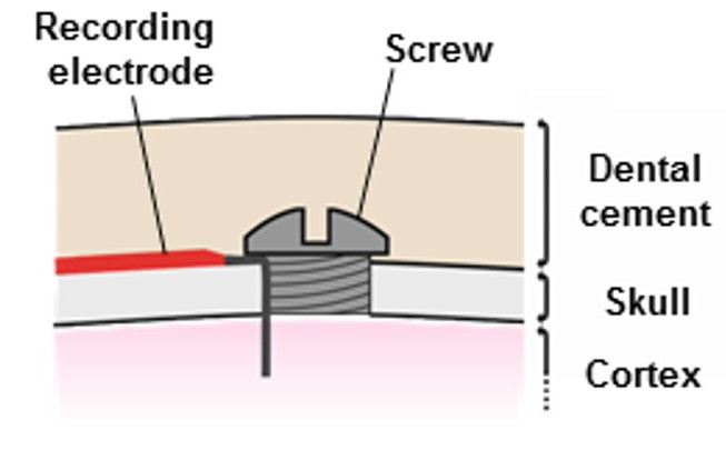
When you first receive an implant, you can ask for it to have exposed, coiled steel wire at the end of its leads. If you want to deploy a bare wire electrode for electrocorticogram (ECoG) recording, ask for the A-Coil termination, which is 1 mm of exposed coil at the end of the lead. When you re-use an implant, you will most likely need to cut a few millimeters off the end of the leads. Now you can make your own A-Coil by removing 1 mm of silicone insulation from the tip of the leads. See Insulation Removal for instructions on how to remove silicone from our spring leads. Once we have exposed 1 mm of coiled wire, we hold the insulated end of the lead with forceps and we grab the exposed wire with tweezers. We stretch and straighten the coil. We put a right-angle bend in the straightened wire and trim the bent section to the desired length. The bend will be at the edge of the skull hole. We trim the bent end to a length equal to the skull thickness plus the distance we want the tip of the wire to penetrate beneath the skull. In rats, we recommend a straightened wire 5.0 mm long with the bend half-way along. In mice, we recommend a 2.4-mm wire with the bend half-way along. We place the bent tip of the wire in a skull hole and lay the insulated lead along the surface of the skull. We thread a screw into the hole. The exposed wire on top of the skull allows the screw to avoid interfering with the silicone insulation of the lead, and will allow dental cement to bond to the wire directly. In rats, the 2.5-mm wire passing through the skull will penetrate roughly 1.0 mm into the brain. In mice, the penetration of the 1.2-mm wire tip will be similar, because the skull is thinner. The wire is held in place by a screw. We cover the screw with dental cement. The cement anchors and insulates the head of the screw, and it bonds to the wire itself.
The electrode lead between the skull and the implant body will flex and stretch as the animal moves around, but the bare wire electrode will be anchored to the skull by its fastening screw. Movement of the brain with respect to the skull will generate movement artifact, but such movements are rare and minimal. We will not see sudden jumps in our iEEG due to intermittent metal-on-metal contact. Nor will we see electromyogram (EMG) from muscles above the screw: we have insulated the top of the screw with cement. A well-secured pair of electrodes produces no more than one or two step artifact per day, while poorly-secured electrodes will produce several artifacts per minute. Step artifacts make it more difficult to apply automatic event detection to our recordings, so we must make every effort to eliminate such corruption of our signals.
We note that there is one stage of the bare-wire implantation procedure that demands care and practice. When we come to securing the bare wire in the skull hole, we need tweezers to hold the screw, a hand to turn the screwdriver, and at the same time the wire must be held in place while we turn the screw into the hole. Here is a description provided by one implanter of how she secures the lead temporarily. "Usually I will put a small amount of cyanoacrylate glue in a small petri dish at the start of the surgery (something like VetBond or MedBond). Then once I've done the burr hole and got the transmitter and place and the hook in the end of the lead, I will place the hook in the burr hole with forceps. Then if you pull down very gently (!) on the transmitter through the skin in the back and pull towards the tail of the animal, it holds the lead in place (if your leads are the correct length). Then while holding like this with one hand, I place a small amount of glue to adhere the wire to the skull (away from the burr hole), with the other hand. By this time the glue becomes tacky as it has been exposed to the air since the start of the surgery. This means it dries quite quickly. Usually holding the transmitter down for around a minute is sufficient. Then you can let go and the lead (usually) stays in place. Then you have both hands to add the screw in place." Here is a suggestion from another implanter about the placement of screws and covering with cement. "Make sure neither screw is anywhere near muscles and that the screws and about half a centimeter of wire coming from the exposed lead is also covered by dental cement so that neither moves at all. I also make completely sure that the cement is very hard before suturing the back incision where the transmitter is so that there is no chance of anything moving before the cement dries."
When we retrieve the transmitter from the animal, we tend to cut the leads where they emerge from the skull cement. It is possible to dissolve dental cement with acetone, as we describe in Silicone and Solvents, but usually the animal's brain is needed intact for examination, so we must cut the leads where they emerge from the head fixture. Having cut the leads, we remove silicone from the tips to expose more wire, as we describe above. Rats and mice scratch at incisions and other points of irritation. The electrode leads of the transmitter, running from the back to the skull beneath the skin of the neck, will irritate the animal if they are poorly routed or if they are too rigid or thick. In one series of experiments, the surgeons found that when the wires were routed directly up the top side of the neck, half the rats scratched the leads out of their skin, which the vets took as a sign of intense discomfort caused by the leads. But when the wires were routed along the side of the neck, with enough slack, none of the rats scratched the leads out. The diagram below shows us how not to route the wires in a rat, and how best to route the wires in a rat.
If we want to inject an agent into the brain, and record iEEG near the site of the injection, we can use a guide cannula to hold the bare wire in place, provided we insulate the wire from the steel shaft of the guide cannula with dental cement. If the steel wire touches the guide cannula, the iEEG amplitude will drop because the steel guide has low electrode impedance. To provide insulation, we cover the bare wire with superglue, cut the end off to expose steel at the tip, bend by 90° and insert in the skull hole. We lower the guide cannula into the same hole, but separated by a few hundred microns from the bare wire, so they do not touch. The following diagram attempts to explain the arrangement.
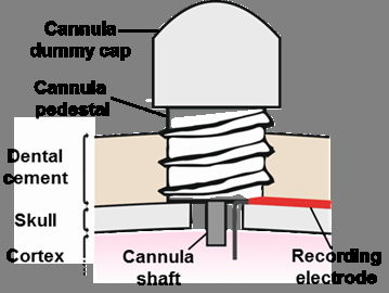
The A3049 and A3047 SCTs come in versions that provide two or more channels each with their own reference, so that we can record potentials in different parts of the body. To record iEEG, EMG, and ECG, for example, we need a three-channel transmitter with six leads. While iEEG is recorded from the brain, and so have the skull available as an anchor, electromyogram (EMG), electrocardiogram (ECG), and electrogastrogram (EGG) are biopotentials generated by soft tissues with no available anchoring bone structure. For these, we use a "soft tissue electrode". Here we present several examples of such electrodes, even though we have picked one as our favorite, which involves threading an "S-Coil" through the tissue and fastening in place with one or two sutures.
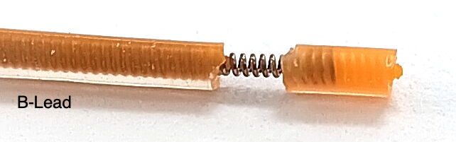
The figure below is an example of ECG recorded with a soft tissue electrode. In this particular case, the ECG used an electrode made out of a P-Coil, a silicone wire cap, and a suture. He cut the leads to the correct length, stretched the final 10 mm of each lead, and cut around the insulation 5 mm from the tip. Once cut, the insulation pulled away from a 1-mm length of wire near the end. He covers the tip with a silicone cap. He fastened the cap in place on the lead tip with a 0/5 silk suture. During surgery, he tied the exposed wires to the thoracic muscle with 0/5 sutures. He placed one wire on one side of the heart and the other diagonally opposite. For a photograph, courtesy of AMU, see Wire_ECG.jpg.
To record electromyogram (EMG), we have two methods recommended by implanters. The first method is the one we recommend for all soft tissue recordings. We begin with an S-Coil. We can make S-Coils on the end of B-Leads, for which the coil is 450 μm in diameter, or C-Leads, for which the coil is 250 μm in diameter. The dimensions of the S-Coil are slightly different for the two leads. On the B-Lead, we can expose 2 mm of bare coil and leave 2 mm of insulation on the tip. On the C-Lead we restrict ourselves to 0.8 mm of bare coil and 1.6 mm of insulation. In both cases, the steel coil ends half-way through the tip insulation. To insert an S-Coil into a muscle, we push a syringe needle through the muscle surface. This needle must be large enough to accommodate the S-Coil insulation easily. Its inner diameter should be around 1.0 mm for the B-Lead S-Coil and 0.7 mm for the C-Lead S-Coil. We slide the S-Coil into the tube so that, within the tube, the S-Coil passes through and out of the muscle. We remove the tube, leaving the S-Coil threaded through the muscle. We suture the lead in place where it enters the muscle, wrapping the suture around the insulation. Where the lead exits the muscle, we can suture the silicone tip in place is we like, or we can trust the one suture to hold the lead securely. We must make sure that no bare wire is visible on either side of the tunnel through the muscle.
Another second EMG method recommended to us, we put a 180° bend at the end of the wire to make a hook. We insert the hook into the muscle, then rotate and pull back to set the tip of the hook in the muscle. We must make sure there is no exposed wire outside the muscle. The insulation must come right up to the muscle surface. Now we secure the lead to the muscle surface with a suture. We place two such hooks in the muscle we want to monitor, or two hooks in a pair of muscles.
To record electrogastrogram (EGG), we use soft tissue electrodes secured to the outer walls of the stomach.
[18-MAR-26] If we end our recording before we exhaust the battery of an implanted transmitter, we can remove our telemetry sensor from the host animal and implant in another animal. We must take care when removing the device, especially if the existing implantation is more than a week old. Scar tissue builds up around the transmitter, holding it in place and wrapping around the antenna and leads. It is easy to cut through the leads or antenna by accident. The ends of the leads are very likely to be fastened in place with dental cement. We can cut the leads where they enter the cement and later remove some silicone from the freshly-cut ends to expose bare steel wire. We describe how to remove silicone insulation from our steel coil leads in our chapter on Insulation Removal. If we are want to attach a screw or pin to the steel wire, we must use acid flux and a hot soldering iron, as we describe in Solder Joints. Attaching your own pins and screws is hard. If you want to save the existing pins and screws attached to the ends of the leads, soak the leads, cement, and the sensor in 20°C acetone for six hours. The cement will dissolve and the leads and sensor will be unharmed. The silicone of the leads and sensor will absorb acetone, but not enough to damage to the structure of the silicone. As we describe in Silicone and Solvents, we must wash the sensor and leads twice with clean acetone after dissolving the cement so as to remove all residue from the silicone surface. Once the sensor and leads are clean, leave them in air for twenty-four hours so that the acetone held by the silicone has time to evaporate. Store your explanted transmitters in a dry place. Do not store in water or any other fluid. Do not store in a container saturated with ethanol or acetone vapor.
When one of our implantable devices exhausts its battery, its operating life is over. There is no way to replace its battery without compromising its reliability. Cutting through the silicone and burning off the epoxy to expose the battery tabs will introduce solder flux into the amplifiers, which will cause the device to fail by corrosion within a few weeks after implantation, or in some cases within a few days. There was a time when we manufactured rechargeable transmitters, but these proved to be pointless. Their operating life was one half that of the non-rechargeable, and any error in the recharging process would lead to premature failure during implantation. Even if we did have a refurbishing system for transmitters, it would be too costly to be worthwhile, when we consider the trouble and cost of shipping them back and forth across international boundaries. For all these reasons we do not manufacture rechargeable implants, nor do we provide any kind of battery replacement or sensor refurbishing service. It is much more cost-effective and far more useful to buy new, long-life devices, implant them repeatedly until they are exhausted, and then buy more devices.
[25-JUN-25] We often want to synchronize our telemetry recordings with events external to the telemetry system. We may, for example, want to know where exactly in our iEEG recording a flash of light occurred. We may want to know when a video recording began or when a noise commenced. We may want to see how the pressure in a plethysmograph, measured with a wired pressure sensor, is related to our recording of EMG from a host animal. In all these cases, we can achieve perfect synchronization by dedicating a telemetry sensor to recording the external event or sensor voltage. Our SCT Interface (A3028BSI) allows us to connect an SCT to a synchronizing signal in a variety of ways. It provides four pairs of spade clips and one BNC socket.
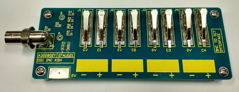
We use the SCT Interface's spade clips to grab wires, in particular the ends of SCT leads. We use the BNC socket to bring in a synchronizing signal with a coaxial cable. The synchronizing signal might take the form of a logic level, it might be a pulse from a trigger system, or it might be mains hum with amplitude that varies when we close a door. The resistors on the A3028BSI allow us to condition our signals for presentation to the SCT leads. The A3028BSI-A, for example, has resistors suitable for logic level synchronization. It provides attenuation of ×1000 from the BNC socket to the clips. A 3.3-V logic transition arriving on the BNC socket will appear as a 3.3-mV step at the SCT input. The A3028BSI-A provides a time constant of 100 μs to remove unwanted high-frequency noise, while at the same time preserving 1-ms synchronization.
| Version | Socket Impedance |
Clip Impedance |
Attenuation (Socket/Clip) |
R1, R2, R3, R4-R7, C1 | Number of Clips |
Application |
|---|---|---|---|---|---|---|
| A3028BSI-A | 10 kΩ | 10 kΩ | 1000 | 10K, 100K, 100R, 10K, 1u0 | 2 | Logic Level Synchronization |
| A3028BSI-B | 51 Ω | 10 MΩ | 100 | 51R, 100K, 1K0, 10M, 100p | 8 | Quad SCT Frequency Sweep Response |
To set up synchronization, we select a transmitter we do not intend to implant. We'll call this the synchronizing SCT. We like to use a large, single-channel, long-life, DC transmitter for synchronization. The A3049L2Z, for example, provides two inputs 0.0-80 Hz and runs continuously for over a year before its battery is exhausted. A DC transmitter like the A3049L2Z allows us to detect DC signals. An AC transmitter has a high-pass filter on its input, so a voltage level step comes out looking like this.
Having chosen our synchronizing SCT, we remove insulation from the lead ends to expose a few millimeters of steel spring coil, and we connect the leads to two of the clips on the SCT Interface. Now we connect our synchronizing signal to the interface as well. We can use two other clips two grab two wires carrying the signal, or we can bring the signal onto the interface with the BNC socket. We turn on the synchronizing transmitter. Our synchronizing signal is being transmitted. We have to make sure we obtain reliable reception of the signal.
If our telemetry system makes use of Faraday enclosures to block local microwave interference, we can put the SCT Interface inside a Faraday enclosure and bring the synchronizing signal into the enclosure with a coaxial cable and one of the coaxial feedthroughs in the enclosure wall. Because we have the synchronizing transmitter in an enclosure, we will obtain reliable reception. Because we are using a coaxial cable and a feedthrough to bring in the synchronizing signal, we will not introduce microwave interference into the enclosure. If our experiment requires that place the SCT Interface outside our Faraday enclosure, we can obtain reliable reception despite local interference by placing the synchronizing transmitter directly on a dedicated antenna. This antenna must be connected to its own, dedicated, telemetry antenna input. Now we have reliable reception because of the proximity of the synchronizing transmitter to antenna, and we have no introduction of interference into the Faraday enclosure because our external antenna is not connected to any antenna inside the enclosures.
Now that our synchronizing transmitter is set up and running, we will see the synchronizing signal in our telemetry recording. If our synchronizing transmitter is a DC transmitter, the signal may be stuck at the bottom or top of the SCT's input dynamic range. If so, the synchronizing signal amplitude is too large or is connected the wrong way around. We must attenuate it so that its transitions are visible. We may have to change some of the resistors on the interface to get the amplitude right. In the end, however, we are sure to figure out some way to get the signal embedded in the SCT input dynamic range, and now its transitions will be recorded in perfect synchronicity with the telemetry recording.
[26-MAY-25] Corrosion is the primary cause of failure for implanted transmitters. Epoxy is water-proof, but it is permeable to water vapor. Any cavities in the epoxy will eventually be filled with condensate. Our encapsulation process is designed to reduce the number of cavities, but we cannot eliminate all cavities. Any residue of solder flux remaining on the circuit board after cleaning provides a space for water to condense and dissolve the residue, creating a surface layer that can conduct electrical charge so as to promote corrosion. Even if there were no cavities in the epoxy, electrical components themselves will eventually corrode in warmth and 100% humidity. Ceramic capacitors, in particular, are prone to cracking during manufacture, assembly and handling. In the warmth and humidity of an animal's body, microscopic cracks in ceramic capacitors corrode until they create an electrically conducting path between the capacitor plates.
We measure the corrosion resistance of every batch of transmitters we produce. We do this by destructive testing of surplus transmitters. If we are shipping twenty transmitters, we will make twenty-four. When all are ready, we will choose two, turn them on, place them in a sealed jar of water, and poach them at 60°C in our oven. We check them every day to see if they are still performing perfectly. If, after one week, they are still running perfectly, we ship the rest of the batch to our customer. If one of them fails, we will re-make the batch and warn our customer that their batch of transmitters will be delayed by two or three weeks.
The poaching is an accelerated aging test for corrosion. According to statistical mechanics, the rate at which a chemical reaction proceeds is proportional to e−E/kT, where T is absolute temperature, E is the activation energy of the rate-determining step in the chemical reaction, and k = 8.6×10⁻⁵ eV/K is the Boltzmann constant. In Hallberg and Peck, the authors show that this relationship applies well to measurements of mean time to failure for temperatures 20-150 °C, relative humidity 20-100%, and activation energy 0.9 eV. Our devices operate at the rodent body temperature of 37°C = 310 K. During our accelerated aging test at 60°C = 333 K, we expect an acceleration of ×10. We are unaware of any corrosion process likely to occur in our circuits that activates with energy less than 0.6 eV. We assume an acceleration of ×10, but we are certain it is at least ×5. One week poaching at 60°C is at least equivalent to 5 weeks implanted.
Today we started with sixteen transmitters poaching in our oven. One of them, an A3048S2, was running when we took it out of the oven, but failed to turn on after we turned it off. This device has been poaching since 11-APR-25, so it lasted 45 days, which is 4 days longer than the minimum operating life we advertise for this model transmitter. Another A3048S, which has been poaching for 39 days, has started generating full-scale, forthy-Hertz oscillations. Oscillations are a sure sign of corrosion in the amplifier. Two others transmitters fail their sweep response test. Both are devices that failed final quality control because we had to burn epoxy off them to replace broken leads. We do not ship such devices because they do not perform well in corrosion tests. The remaining eleven devices turn on and off, report an accurate battery voltage, and give us the correct sweep response. We put fifteen transmitters back in the oven and set aside the exhausted device as a physical sample.
[30-JUL-25] In the Appendix to our Telemetry Manual, you will find the following chapters:
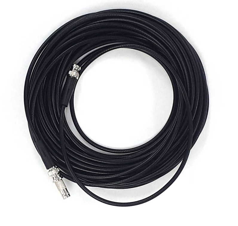
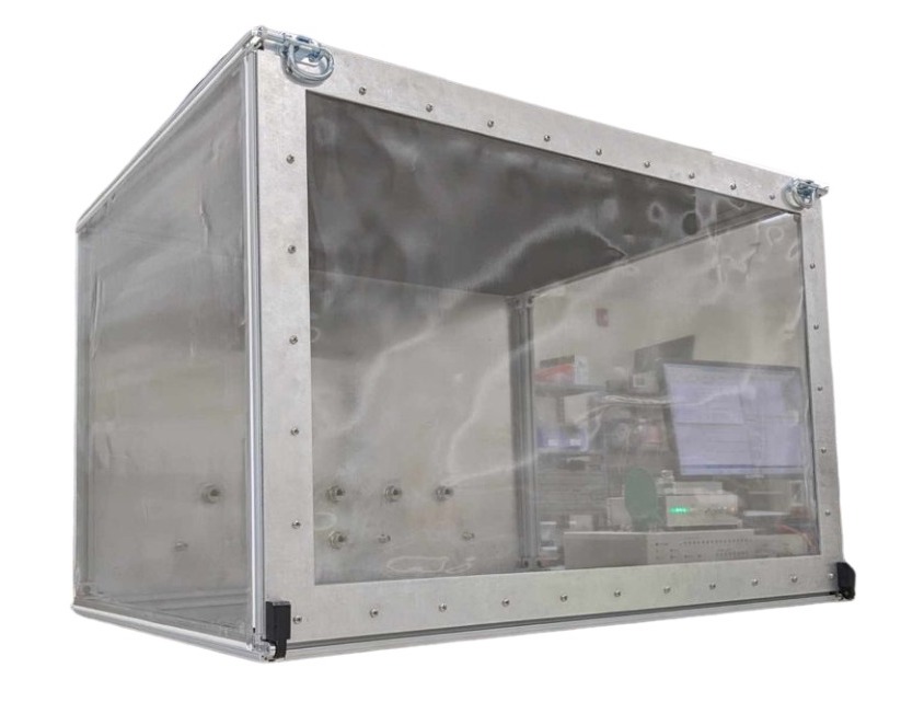
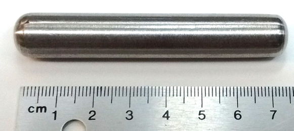
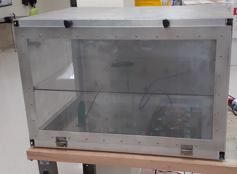
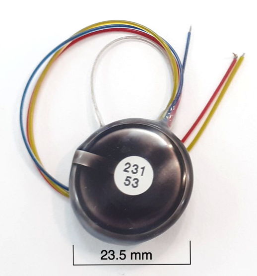
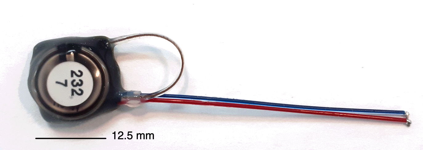
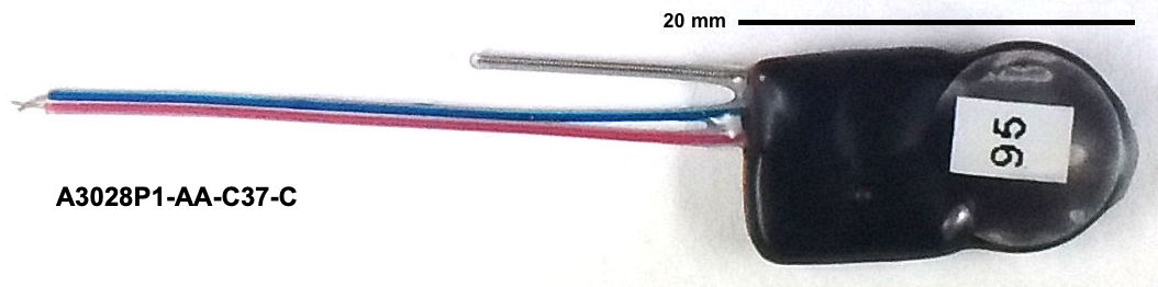
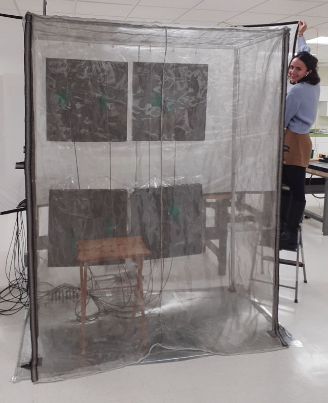
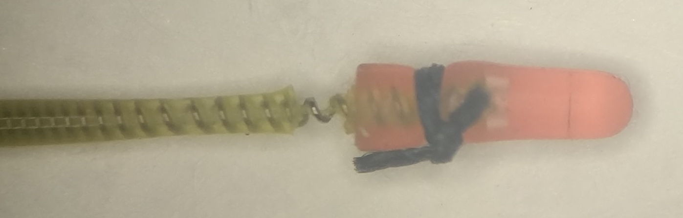