[18-JUL-25] The Event Classifier in the Neuroplayer Tool provides automatic detection of a wide variety of events in local field potential (LFP) and electroencephalograph (EEG) recordings. It operates upon signals recorded from our Subcutaneous Transmitters (SCTs) and Head-Mounting Transmitters (HMTs). These telemetry devices provide high-fidelity EEG, EMG, ECG, and EGG from live, freely-moving laboratory mice and rats. Our objective is to detect rare events in continuous recordings. We count these events, measure their duration, or respond to them with a real-time stimulus delivered to the subject animal. We may have one hundred thousand hours of EEG from a fifty animals and we want to count inter-ictal spikes that occur roughly once per hour with a precision ±0.1 spike per hour, which means our detection algorithm must generate no more than one false spike detection per ten hours. That is: the probability of a false positive in any one interval must be of order 0.001%. In order to achieve such a low false positive rate, the EEG recording must be free of movement artifact, devoid of electrical noise, and uninterrupted by wireless reception failure. The success of the event detection algorithms is founded upon the high fidelity of the recordings we obtain from our SCTs and HMTs. We describe our latest event-detection metrics in the Event Classification chapter. Roughly half the users of our Subcutaneous Transmitters (SCT) system use the Event Classifier to analyze their data. There are users of other telemetry systems who translate their recordings into our NDF format so that they can make use of our Event Classifier to perform their analysis.
Reception of wireless messages from a moving animal cannot be 100% reliable, but it can come close. Before you begin a study, we recommend you ensure that your telemetry system is set up correctly and reception from freely-moving animals is at least 98%. Pick the best electrode, and establish a procedure for securing the electrodes in place to avoid movement artifact. We discuss our choice of electrodes in Electrodes and Terminations. We present our own understanding of the sources of EEG in The Source of EEG. For example recordings, see Example Recordings.
[18-JUL-25] By baseline signal we mean an interval of EEG that does not contain any unusual event. This definition is vague, and proves to be difficult to define in the logic of seizure detection. In order to identify a baseline interval, for example, we must be sure we are able to identify all unusual events. A baseline interval an interval that contains no such events. If we are confident in our ability to identify baseline signal by eye, we can find such intervals ourselves, and so measure their amplitude. The define baseline amplitude to be the amplitude of a baseline interval. We discuss strategies for identifying baseline intervals automatically in our Baseline Calibration chapter.
| Animal | Electrode | Location | Bandwidth (Hz) |
Amplitude (μV rms) |
|---|---|---|---|---|
| rat | steel screw | cortex, on surface | 160 | 50 |
| rat | bare wire | cortex, under surface | 160 | 100 |
| mouse | steel screw | cortex, on surface | 160 | 20 |
| mouse | bare wire | cortex, under surface | 160 | 40 |
| mouse | bare wire | cortex, under surface | 40 | 35 |
| mouse | insulated wire | hippocampus | 160 | 80 |
The following shows a four-second interval of EEG from eight separate control rats recorded at ION/UCL. We have fifteen hours of control recordings in archives M1297634713 through M1297685113 made on 14-FEB-11. The animals have recovered from surgery and have received no drugs. The electrodes are soldered screws held in place and insulated with dental cement.
The amplitude of these control signals varies from 30 μV to 80 μV rms in two-second intervals. During the course of ten minutes, the average amplitude of all eight signals in four-second intervals is between 40 μV and 60 μV. We calculate the signal power in three separate frequency bands for these control recordings using the following interval processor. The bands are transient (0.1-1.9 Hz), seizure (2.0-20.0 Hz), and burst (60.0-160.0 Hz).
set config(glitch_threshold) 1000
append result "$info(channel_num) [format %.2f [expr 100.0 - $info(loss)]] "
set tp [expr 0.001 * [Neuroplayer_band_power 0.1 1.9 0]]
set sp [expr 0.001 * [Neuroplayer_band_power 2.0 20.0 0]]
set bp [expr 0.001 * [Neuroplayer_band_power 60.0 160.0 0]]
append result "[format %.2f $tp] [format %.2f $sp] [format %.2f $bp] "
The Neuroplayer_band_power routine returns one half the sum of squares of the amplitudes of all the Fourier transform components within a frequency band. We call this the band power. The filtered signal is the signal we would obtain by taking the inverse transform of the frequency spectrum after setting all components outside the frequency band to zero. We define the amplitude of the filtered signal to be its root mean square value. The amplitude is A√p, where p is the band power and A is a conversion factor in μV/count. The AC-coupled versions of our SCT and HMT sensors have A = 0.45 μV/count. If the band power is 5000 square-count, or 5000 sqcnt, or 5 ksqcnt. The amplitude of the filtered signal is 32 μV. In the script above we calculate power in three bands. The transient band is from 0.1-1.9 Hz. It captures movement artifact. The seizure band is 2.0-20 Hz. It captures the power of epileptic seizures. The burst band is 60-0160 Hz. It captures high-frequency bursts, such as occur in the tetanus toxin model of epilepsy. We use an interval analysis program called Power Band Average (PBAV4.tcl) to obtain the average power in the transient band every minute for two transmitters implanted in rats.
The transient amplitude is always less than 25 μV rms during any one-minute period and usually 7 μV rms. When the electrodes are loose, however, we see transient spikes on the EEG signal that are caused by movement of the electrodes with respect to the brain. We use our Transient Spike (TS) interval analysis to search for transient amplitude greater than 63 μV and by this means we are able to count transients like this and this. We plot the average power in the seizure band per minute for two implanted transmitters, the same ones for which we plotted transient band power above. The seizure-band amplitude varies from 18 μV rms to 45 μV rms.
In a recording made with insecure electrodes, the seizure-band power will corrupted by transients, as you can see here. Burst-band power, however, is far less affected by transients, as you can below.
The baseline signal amplitude obtained from screws in a rat's skull is around 35 μV rms in the 1-160 Hz band, 18 μV in 2-20 Hz, and 9 μV in 60-160 Hz. When the amplitude in the 0.1-1.9 Hz band rises above 70 μV, it is likely that the electrodes are generating a transient spike. In the absence of any transient spikes, the amplitude of the 2.0-20.0 Hz band has a minimum amplitude of around 20 μV rms, and rises to 40 μV for an hour or two at a time.
[30-OCT-18] Our transmitters can provide a variety of bandwidths for biopotential recording. The sample rate required to implement the bandwidth is proportional to the high-frequency end of the bandwidth. A 0.3-40 Hz bandwidth requires 128 SPS (samples per second), while a 0.3-640 Hz bandwidth requires 2048 SPS. Increasing the sample rate increases the operating current of the device, and therefore decreases its battery life. See here for examples of sample rate, volume, and operating life.
In order to obtain the longest operating life from an implanted transmitter, we must use the smallest bandwidth that will permit us to observe the events we wish to assess. When we design an experiment to count epileptic seizures, for example, we can start by implanting a transmitter with a bandwidth large enough that we are certain to record every feature of the seizure, and then examine our recordings to see if a smaller bandwidth will be sufficient. The following processor script applies a band-pass filter to a signal during playback so we can see how a signal will look with a smaller bandwidth.
# Calculate power in the band f_lo to f_hi in Hertz. Plot the signal as it
# would look if filtered to this range.
set f_lo 0.3
set f_hi 40.0
set power [Neuroplayer_band_power 0.1 $f_hi 1]
append result "[format %.2f [expr sqrt($power)*0.4]] "
In the figure below, we see an eight-second interval of EEG containing a seizure confirmed by video. The original signal was recorded at 512 SPS with bandwidth 0.3-160 Hz. We see this signal displayed along with a 40-Hz low-pass filtered version of the same signal.
The example above shows that the prominent spikes of the seizure are visible in both the 160-Hz and 40-Hz bandwidths. We could detect such seizures with a transmitter operating at 0.3-40 Hz and 128 SPS.
The interval above shows what we believe is grooming artifact in an EEG signal. The burst of 80-100 Hz power is EMG being introduced into the EEG signal through the skull screw electrodes. We can see the grooming artifact clearly in the 160 Hz signal, but in the 40-Hz signal, the grooming is lost among the other fluctuations, so that we would be unable to count such artifacts, or guarantee that they are not affecting our EEG recording.
The interval above shows a short, solitary spike in mouse EEG. The spike is short and sharp. The 40-Hz bandwidth doubles the width of the base of the spike, but does not prevent us from seeing the spike clearly.
[12-APR-10] We have five hours of data recorded at the Institute of Neurology (ION) at University College London (UCL) by Dr. Matthew Walker and his student Pishan Chang using the A3013A. The inverse-gain of this transmitter is 0.14 μV/count. Here we consider using the ratio of band powers to detect seizures. Using a power ratio has the potential advantage of making seizure detection independent of the sensitivity of individual implant electrodes.
When we tried to detect seizures by measuring power in the range 2-160 Hz, we found that step-like transient events also produced high power. We're not sure of the source of these transients, but we suspect they are the result of intermittent contact between two types of metal in the electrodes. We are sure they are not seizures.
We define a seizure band, in which we expect epileptic seizures to exhibit most of their their power, and a transient band, in which we expect transient steps to exhibit power. In our initial experiments we choose 3-30 Hz for the seizure band and 0.2-2 Hz for the transient band. Seizures show up as power in the seizure band, but not in the transient band. Transients show up as power in both bands. When we see exceptional power in the seizure band, and the seizure power is five times greater than the transient power, we tag this interval as a candidate seizure. You can repeat our analysis with the following script.
set seizure_power [Neuroplayer_band_power 3 30 $config(enable_vt)]
set transient_power [Neuroplayer_band_power 0.2 2 0]
append result "$info(channel_num)\
  [format %.2f [expr 0.001 * $seizure_power]]\
  [format %.2f [expr 1.0 * $seizure_power / $transient_power]]"
if {($seizure_power > 1000000) \
  && ($seizure_power > [expr 5.0 * $transient_power])} {
  Neuroplayer_print "Seizure on $info(channel_num) at $config(play_time) s." purple
}
The following graphs show seizure-band power and seizure-transient power ratio for the first hour of our recording (M1262395837). We used window fraction 0.1 and glitch filter threshold 10,000 (1.4 mV). The playback interval was 4 s.
In these recordings, we convert band power to filtered signal amplitude with a = √(p/2) * 0.14 μV/count. Our seizure power threshold of 1 Msqcnt is the same as a seizure-band amplitude threshold of 100 μV. Our requirement that the seizure power be five times the transient power is the same as requiring that the seizure-band amplitude ba 2.2 times the transient-band amplitude.
Only the seizure activity confirmed by Dr. Walker on No1 has both high seizure power and high power ratio. There are sixteen 4-s intervals between 1244 s to 1336 s that qualify as seizures according to our criteria, and Dr. Walker agrees that they are indeed seizures. Channels No2 and No3 have many intervals with glitches and transients, but no seizures. Channel No7 has high power ratio in places, and at these times the signal looks like a seizure, but the power is below our threshold.
We apply the same processing to the remaining four hours of recordings. We see several more confirmed seizures on No1 up to a hundred seconds long. We see a few seizure-like intervals on No3 and No7. We cannot confirm whether these are short seizures or other activity. The following figure gives an example of such an interval.

Power ratios are useful in isolating seizures from the baseline signal, but we have been unable to isolate seizures using power ratios alone. In practice, we may have to rely upon consistency between implant electrodes so that we can use the amplitude of the signal as an additional isolation criterion.
[27-FEB-25] By default, the Neuroplayer calculates the discrete Fourier transform of each interval it processes. We can write the entire spectrum to a characteristics file with the following processor. Copy and paste this one line into a text file and use it as your processor script to produce the spectrum characteristics file.
append result "$info(channel_num) $info(spectrum) "
The spectrum will consist of NT real-valued numbers, where N is the number of samples per second in the original signal, and T is the length of the interval. The numbers are arranged in pairs, numbered k = 0 to NT/2−1. The k'th pair specifies the amplitude and phase of the k'th component of the transform. The frequency of this component is k/T. The first number in the pair is the amplitude in ADC counts and the second number is the phase in radians. The k = 0 pair is an exception: the first number is the 0-Hz amplitude, which is the average value of the signal, while the second number is the N/2-Hz amplitude and phase. If this amplitude is positive, the phase of the N/2-Hz component is zero, if negative its phase is π.
Example: We save the spectrum of a 1-s interval of 512 SPS. We have N = 512 and T = 1. There are 512 numbers in the transform, arranged as 256 pairs, and representing the components from 0 Hz to 256 Hz. The first pair, which is the k = 0 pair, specifies the 0-Hz and 256-Hz components. The k > 0 pairs specify the amplitude and phase of the components with frequency k Hz. We switch to 8-s intervals. Now we have N = 512 and T = 8. The spectrum contains 4096 numbers arranged as 2048 pairs, with components 0-256 Hz in 0.125-Hz increments. The first pair still represents the 0-Hz and 256-Hz components. The k'th pair represents the component with frequency k/8.
[More practical than writing all components of the spectrum to the characteristics file is to write a set of band powers. We obtain a measure of the power of the signal within a frequency range, we sum the squares of amplitudes of the components that lie within the range and divide by two. The result is the average band power, in units square-count, or sqcnt. We call this the band power. The following processor calculates the power in 39 contiguous bands between 1 and 40 Hz.
append result "$info(channel_num) [Neuroplayer_contiguous_band_power 1 40 39] "
To convert the band power to μV2, determine the ratio μV/count for the transmitter that made the recording. For most A3028 transmitters, this ratio is 0.4 μV/count. To convert from sqcnt to μV2, we multiply by 0.16 μV2/sqcnt. To obtain the root mean square amplitude of the signal contained in a band, take the square root of the band power and multiply by 0.4 μV/count to obtain μV rms.
If we want to define our own set of bands for our spectrograph, we can do so with the Neuroplayer_band_power routine applied repeatedly to our own frequency boundaries. If we want the coastline of our signal, we can use lwdaq coastline_x applied to the signal sample values. The following script illustrates both calculations.
# Obtain the coastline of a signal in units of kcnt. Obtain the power in bands
# 1-4, 4-12, 12-30, 30-80 Hz, where each band includes the lower boundary but
# not the upper boundary. Power units are ksqcnt. Set all values to zero if
# signal loss is greater than 20%.
set max_loss 20.0
append result "$info(channel_num) "
if {$info(loss) <= $max_loss} {
	set cl [lwdaq coastline_x $info(values)]
} else {
	set cl "0.0"
}
append result "[format %.1f [expr 0.001 * $cl]] "set f_lo 1.0
foreach f_hi {4.0 12.0 30.0 80.0} {
	if {$info(loss) <= $max_loss} {
		set bp [Neuroplayer_band_power [expr $f_lo + 0.01] $f_hi 0]
	} else {
		set bp 0.0
	}
	append result "[format %.2f [expr 0.001 * $bp]] "
	set f_lo $f_hi
}
Once you have a characteristics file with the spectrum of the signal recorded in sufficient detail, you can plot the spectrum versus time in a spectrograph, whereby the evolution of power with time is recorded using a time axis, a frequency axis, and a color code for power in the available bands. The PC1 processor calculates the coastline of each interval and the power in a set of bands specified by low and high frequencies in the processor script. Unlike the script above, this processor allows you to specify frequency bands that overlap or have gaps between them. When this processor encounters a line with loss, it writes blank values to the result string, separated by spaces, so that pasting the characteristics into a spreadsheet will produce blank cells that are automatically excluded from sums. Furthermore, the processor allows us to specify a low-pass filter we can apply to the signal before calculating the coastline.
[12-APR-10] The EEG signals recorded at UCL from epileptic rats contain bursts of power in the range 60-100 Hz, with several bursts per second. The figure below gives an example.
The inverse-gain of the A3013A is 0.14 μV/count, so the burst has peak-to-peak amplitude of 500 μV. The following figure shows the same signal for a longer interval, showing how the bursts are repetitive.
We used the following processor script to detect wave bursts as well as seizures.
set seizure_power [expr 0.001 * [Neuroplayer_band_power 3 30 0]]
set burst_power [expr 0.001 * [Neuroplayer_band_power 40 160 $config(enable_vt)]]
set transient_power [expr 0.001 * [Neuroplayer_band_power 0.2 2 0]]
append result "$info(channel_num)\
  [format %.2f $transient_power]\
  [format %.2f $seizure_power]\
  [format %.2f $burst_power] "
if {($seizure_power > 1000) \
  && ($seizure_power > [expr 5.0 * $transient_power])} {
  Neuroplayer_print "Seizure on $info(channel_num) at $config(play_time) s." purple
}
if {($burst_power > 100) \
  && ($burst_power > [expr 0.5 * $transient_power])\
  && ($burst_power > $seizure_power)} {
  Neuroplayer_print "Wave burst on $info(channel_num) at $config(play_time) s." purple
}
The wave bursts on No3 in M1264098379 come and go for periods of a minute or longer. They are spread throughout the archive. When they occur, they often do so at roughly 5 Hz, but not always. In places, such as time 40 s, a single burst endures for a full second.
[09-JUN-10] The above script is effective at detecting all wave bursts, but it also responds to glitches too small for our glitch filter to eliminate. These glitches, caused by bad messages, were common before we introduced faraday enclosures and active antenna combiners to the recording system. Wave bursts are easy to detect using the 160-Hz bandwidth of the A3013A and A3019D.
[08-SEP-11] These wave bursts are most likely eating artifacts, which we have since seen in many other recordings.
[01-DEC-25] To export data from SCT recordings, use the Neuroplayer's Exporter. The Exporter allows us to specify any time span in a continuous recording to write to disk either as a binary or text file. The Exporter performs signal reconstruction before exporting, so as to guarantee a fixed number of samples per second. We can execute an interval processor while we export. We could, for example, apply a low-pass filter to our signals before export by using a low-pass filter processor. The Exporter combines video files to make a continuous videos that match the exact span of your exported telemetry data, starting at the same moment and ending at the same moment.
We recommend you use the Neuroplayer's Exporter for all your export projects, great and small. Use multiple Exporters to speed up the process: launch separate Neuroplayers from your original LWDAQ process, and open the Exporter panels in each of them. These Exporters will all operate independently and you can assign an equal portion of your export task to each of them. If you have ten weeks of telemetry recordings to translate, launch five Exporters and export two weeks of recordings with each of the five. Consult the Exporter Manual to see how you can define the start and end time of each export, and how you can export two weeks of telemetry recordings into fourteen twenty-four-hour long export files with a single Exporter. Running multiple Exporters in parallel will be effective only if the computer upon which you are performing the exports is equipped with multiple processor cores and multiple caches for its hard drives, but assuming you are running on an eight core desktop machine, or even a Linux cluster, you will be able to get your export done five times as fast with five Exporters.
If you are adept at command-line programming, and you want to translate NDF files into EDF files according to some regular schedule, or you have a very large number of files to translate and you do not want to clutter your desktop with Exporter panels, consider using our command-line NDF-to-EDF Translation Management System. This system is managed by ndf2edf.tcl with the help of ndf2edf_config.tcl to configure export processes and ndf2edf_processor.tcl to perform the actual translation and storage. All three of these scripts work together to provide translation from NDF to EDF, and even concatination of EDF files after translation. The following is an example of a terminal command that launches the ndf2edf system:
~/LWDAQ/lwdaq --no-gui ~/TestA/ndf2edf.tcl -S1447073970 -P4 -m -c -q'1:512 5:512 9:256 51:256'
We give an absolute path to both the LWDAQ shell and the NDF directory. When we run the above command, it will commence translation and export of NDF files in the directory tree containing the ndf2edf.tcl, which in this case is ~/TestA. It will begin the export with a file that has a start time equal to or greater than 12:59:30 GMT on 09-NOV-15 (UNIX time 1447073970). It will select channel numbers 1, 5, 9, and 51 with sample rates 512, 512, 256, and 256 SPS respectively. The manager will use up to four threads to run the file-translation processes (-P4). If our computer has four or more cores, we might hope for all four threads to run in parallel and at full speed. On our hard drive, we will see four EDF files growing at the same time. Nowhere in the above command do we specify the dynamic range of the telemetry signals. This specification must be performed by editing the translation processor script itself. If you leave the translation processor unchanged, it will translate all signals as sixteen-bit unsigned integers. You can apply dynamic ranges in your EDF viewer later. But if you want the scaling and units in place at the time of translation, take a look at ndf2edf_processor.tcl and read the comments. For a complete description of how to set up and run the NDF-to-EDF we refer you to the comments at the top of ndf2edf.tcl and ndf2edf_config.tcl. For a description of the translation calculations, we refer you to the comments within ndf2edf_processor.tcl.
If we want to export a sample of one of our recordings for the purposes of plotting for presentation, we like to use a Neuroplayer interval processor that extracts the signals as we play them in the Neuroplayer and stores them in a text file. We navigate to the interval we want to export, we enable the interval processor, we press Step in the Neuroplayer until we have moved all the way through the sample we want to export. Now we have all the samples from the segment in a text file and we can load them into our plotting program. The following processor fulfills this function for us: it appends the signal from channel n to a file En.txt in the same directory as the NDF file. It even allows us to apply a low-pass filter to the data before exporting, with the help of Neuroplayer_band_power routine.
# Sample Exporter for Presentations and Plots
set fn [file join [file dirname $config(play_file)] "E$info(channel_num)\.txt"]
Neuroplayer_band_power 0.0 80.0 1 1
set export_string ""
foreach value $info(values) {
  append export_string "[format %.1f $value]\n"
}
set f [open $fn a]
puts -nonewline $f $export_string
close $f
This sample exporter goes through all active channels and writes the sixteen-bit sample values to the text file dedicated to each channel. Each sample value appears on a separate line. By "active channels" we mean those specified by the channel selector string. Before export, the Neuroplayer will perform reconstruction and glitch filtering upon the raw data. Reconstruction attempts to eliminate bad messages from the message stream and replace missing messages with substitute messages. We describe the reconstruction process in detail here. Reconstruction always produces a messages stream fully-populated with samples, regardless of the number of missing or bad message in the raw data. Glitch filtering will be enabled only if we have set the glitch threshold to a value greater than zero. The "1 1" tell the band-power routine to plot the filtered signal and to over-write the existing signal values with the filtered signal values.
If we want to export the spectrum of a signal, instead of calculating the spectrum ourselves using an export of the original signal, we can do so with a interval processor. The following interval processor stores all components of the discrete Fourier transform to a file named Sn.txt in the same directory as the NDF archive, where n is the channel number. An eight-second interval recorded from a 512 SPS transmitter will contain 4096 samples. We can represent these with 2048 sinusoidal components and a constant offset. When we export the spectrum, we store the constant offset in the first line, as the 0-Hz component. The final line is the 2048'th frequency component (not counting 0-Hz). The script does not store the phases of the sinusoids. The amplitudes of all components are positive numbers.
set fn [file join [file dirname $config(play_file)] "S$info(channel_num)\.txt"]
set export_string ""
set f 0
set a_top 0
foreach {a p} $info(spectrum) {
	append export_string "$f $a\n"
	if {$f == 0} {set a_top $p}
	set f [expr $f + $info(f_step)]
}
append export_string "$f [expr abs($a_top)]\n"
set f [open $fn a]
puts -nonewline $f $export_string
close $f
append result "$info(channel_num) [expr [llength $export_string]/2] "
Our Periodic_Export.tcl processor exports only occasional intervals to disk: we define a period for export, such as 180 seconds, and one interval in every 180 s will exported to the disk file. If our interval length is 1 s, we will have 1 s out of every 180 s recorded to the export file. The export file is a text file, and each interval is written to one line. That line begins with a UNIX timestamp and is followed by signal values. If the interval has signal loss higher than a threshold specified in the script, the interval is not written, but is skipped entirely.
Some of our customers like to view telemetry signals in the LabChart software provided by ADInstruments. We claim that our LabChart_Exporter.tcl interval processor exports NDF recordings in a form that the Lab Chart program can read in and display. Follow the instructions in the comments at the top of the interval processor and see if the translator works. If not, let us know and we might be able to figure out what new feature of LabChart is preventing the export from being readable.
[10-FEB-20] Suppose we have twenty-four thousand one-hour NDF files, and we want to re-arrange them as one thousand 24-hr NDF files. That is: we want to concatinate consecutive NDF recordings into longer recordings. Our NDF Concatination script is a LWDAQ Toolmaker script that will perform the concatination for you in one pass, after the hour-long NDF files have been recorded. Place all the NDF files in the same directory. Copy and paste the script into an empty Toolmaker window and press Execute. The program asks you to specify the directory containing the NDF files, and then creates beside this directory another directory into which it will write the concatinated files. During the concatination process, no files will be deleted. If your concatination directory contains some NDF files before you run the concatination script, the process will abort with an error. Our objective is to avoid over-writing or otherwise corrupting your recordings. Any deletion of files you will do yourself.
[04-AUG-22] Our TDT1 (Text Data Translator, Version One) transforms text data into the NDF format. It runs in the LWDAQ Toolmaker. The script creates a new NDF file and translates from text to binary NDF sample format. It inserts the necessary timestamp messages. Each line in the input text file must have the same number of voltage values. A check-button in the TDT1 lets you delete the first value if it is the sample time. The values can be space or tab delimited. The translator assigns a different channel number to each voltage. It allows us to specify the the bottom and top of the dynamic range of the samples. The range will be mapped onto the subcutaneous transmitter system's sixteen-bit integer range. The translator requires us to specify a sample rate for the translation. The Neuroplayer is more robust when working with sample rates that are a perfect power of two, but TDT1 will open and configure the Neuroplayer to play an archive with any sample rate. We set the Neuroplayer's playback interval to some value between 1 s and 2 s that includes a number of samples that is a perfect power of two. If the sample rate is 1000 SPS, we set the play interval to 1.024 s, so we will see 1024 samples per interval.
[10-OCT-12] We update our original TDT1 translator. The translator does not read the entire text file at the start, but goes through it line by line, thus allowing it to deal with arbitrarily large files. It writes the channel names and numbers to the metadata of the translated archive.
[20-MAY-10] We receive from Sameer Dhamne (Children's Hospital Boston) a text file containing some EEG data they recorded from an epileptic rat. The header in the file says the sample rate is 400 Hz and the units of voltage are μV. There follows a list of 500k voltages, which covers a period of 1250 s. He asked us to import the data into the Neuroplayer and try our seizure-finding algorithm on it.
We remove the header from the file we received from Sameer and apply our translator. Our Fourier transform won't work on a number of samples that is not a perfect power of two, and our reconstruction won't work on a sample period that is not an integer multiple of the 32.768 kHz clock period. We don't need the reconstruction, since this data has no missing samples. So we turn it off. We use the Neuroplayer's Configuration Panel set the playback interval to a time that contains a number of samples that is an exact power of two. We now see the data and a spectrum.
[21-MAY-10] Our initial spectrum had a hole in it at 80 Hz, when we expect the hole to be at 60 Hz. We obtain the transform of the text file data using the following script, and plot the spectrum in Excel. We see a hole at 60 Hz.
set fn [LWDAQ_get_file_name]
set df [open $fn r]
set data [read $df]
close $df
set interval [lrange $data 0 4095]
set spectrum [lwdaq_fft $interval]
set f_step [expr 1.0*400/4096]
set frequency 0
foreach {a p} $spectrum {
  LWDAQ_print $t "[format %.3f $frequency] $a "
  set frequency [expr $frequency + $f_step]
}
We correct a bug in the translator, whereby we skip a sample whenever we insert a timestamp into the translated data, and our imported spectrum is now correct, as you can see below.

According to Sameer, the text data was recorded from a tethered rat. Here we see 5.12 s of the signal displayed, and its spectrum. There is a 60 Hz mains stop filter operating upon the signal. We see what appears to be an epileptic seizure taking place. This interval covers 1034 s to 1039 s from the start of the recording.
[19-JUN-11] We receive two text files from Sameer Dhamne (Children's Hospital Boston). They represent recordings made with tethered electrodes. Each line consists of a time, a comma, and a sample value. We assume the time is seconds from the beginning of the file and the sample is in microvolts. The samples occur every 2.5 ms for a sample frequency of 400 Hz. We give our text files names of the form Mxxxxxxxxxx.txt so that the TDT1 script will create archives of the form Mxxxxxxxxxx.ndf, which is what the Neuroplayer expects.
We run the TDT1 script. We set the voltage range to ±13000 in the text file's voltage units. Because we assume the unit is μV, our range is therefore ±13 mV, which is the dynamic range of an A3019. We produce two archives, one 300 s and the other 600 s long. The script sets up the Neuroplayer to have default sample frequency 400 Hz and playback interval 1.28 s. These combine to create an interval with 512 samples, which is a perfect power of two, as required by our fast Fourier transform routine. We play back the archive and look for short seizures. Before we can return to play-back of A3019 archives, we must restore the default configuration of the Neuroplayer, such as sampling frequency of 512 SPS. The easiest way to do this is to close the Neuroplayer window and open it again.
[11-FEB-12] Our new TDT3 script allows us to extract up to fourteen signals from a text file database. The first line of the text file should give the names of the signals, and subsequent lines should give the signal values. There should be no time information in the first column. Instead, we tell the translator script the sample rate. We also tell it the full range of the signals for translation into our sixteen-bit format. We used this script to extract human EEG signals from text files we received from Athena Lemesiou (Institute of Neurology, UCL).
[27-APR-12] Our new TDT4 script allows us to extract all channels from a text file database and record them in multiple NDF files, with up to fourteen channels in each NDF file. The first line of the text file should give the names of the signals, and subsequent lines should give the signal values. The script records in the metadata of each NDF file the channel names and their corresponding NDF channel numbers within the NDF file. As in TDT3, we can set the full range of the signals for translation into our sixteen-bit format. Copy and paste the script into the LWDAQ Toolmaker and press Execute. The program is not fast: it takes two minutes on our laptop to translate ten minutes of data from sixty-four channels.
[10-APR-13] We improve TDT1 so that it records more details of the translation in the ndf metadata. We fix problems in the Neuroplayer that stopped it working with translated archives of sample rate 400 SPS.
[28-JAN-16] A correspondant in the Netherlands uses TDT1 to translate a recording made with an ETA-F10 implantable monitor manufactured by DSI. His hope is to perform seizure detection with the Event Classifier. He applies a sinusoidal input to the device at frequencies 1 Hz, 5 Hz, 10 Hz, 20 Hz, 50 Hz, 100 Hz, 200 Hz, 500 Hz, 1000 Hz. The sample rate of the original signal is 1000 Hz, which we scale to 1024 Hz so we can apply a fast fourier transform to a one-second interval.
The spectrum of the 1-Hz fundamental is shown in here. Instead of a single peak at the fundamental frequency, we have a smeared peak after the fashion of a 1-Hz signal transmitted by frequency modulation. The ETA-F10 appears to emit pulses at a nominal frequency of 1 kHz, and modulates their frequency to indicate the signal voltage. The high-frequency artifact added to the sinusoid by the ETA-F10 has frequency 450-520 Hz. Because this artifact is greater on negative cycles of the sinusoide, it could easily be mistaken for a high frequency oscillation in the EEG. Knowing that this artifact exists, we can remove it with a 200-Hz low-pass filter. What remains below 200 Hz is a mild distortion of the 1-Hz waveform.
# Processor script to low-pass filter signal to 200 Hz.
Neuroplayer_band_power 0.1 200 1
scan [lwdaq ave_stdev $info(values)] %f%f%f%f%f ave stdev max min mad
append result "$info(channel_num) [format %.2f [expr 100.0 - $info(loss)]]\
	[format %.2f [expr 1.8*65536/$ave]] [format %.1f $stdev] "
As we increase the frequency of the sinusoid, the amplitude of the signal drops as if there is a single-pole low-pass filter acting on the signal with corner frequency 100 Hz. At 200 Hz, we see distortion of the signal by a combination of modulation and aliasing, as is evident in the spectrum. The fundamental at 200 Hz is accompanied by another waveform at 290 Hz, and lower-frequency distortion at 50 Hz and 90 Hz.
Given that most interesting features in EEG are below 100 Hz, we recommend a pre-processing low-pass filter at 100 Hz for event detection in ETA-F10 recordings. A 100-Hz low-pass filter will remove most distortion of an EEG signal. When transients occur due to loss of signal or electrode movement, the high-frequency power in these steps will emerge from modulation and aliasing as low-frequency artifacts. A 100-Hz low-pass filter will not eliminate such artifacts.
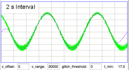
[25-MAY-17] At the end of one of the recordings we have from an ETA-F10 transmitter made by DSI (see above), the animal dies. Following its death, we observe the following signal from the ETA-F10.

The above signal is the noise generated by an ETA-F10 while stationary in a conducting body. When the animal is alive, the baseline EEG amplitude is 25 μV rms.
[22-JUN-26] The electrocardiogram (ECG) waveform is a sequence of spikes that are easy to record. We can measure heart rate in two ways: by finding spikes and measuring their average separation in time, or by taking the Fourier transform and finding the fundamental frequency of the spike train in the spectrum.
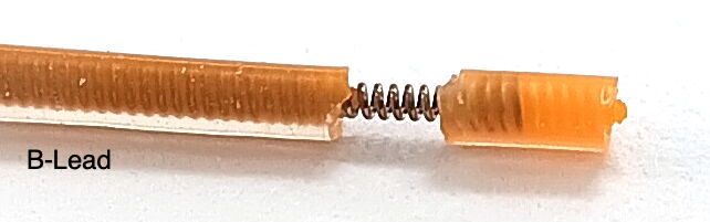
We record ECG with what "soft tissue electrodes", or "S-Coils". We will fabricate S-Coils for you on the end of your ECG leads. If you re-implant a transmitter, however, you may have to cut back the lead during explantation. If so, you can fabricate S-Coils for yourself using a scalpel. We describe how to attach an S-Coil to a muscle on our Electrode Surgery Protocols page. Implant one electrode on one side of the heart and the other diagonally opposite, inside the thoracic cavity.
When we record ECG we are often able to pick up a respiration signal as well. In the figure Electrocardiogram and Respiration we see a four-second interval from a recording made by two electrodes running through an incision in the torso of an unconcious rat. When we look at the spectrum from 0-10 Hz in more detail, we can see clearly the first, second, and third harmonics of respiration at 1, 2, and 3 Hz respectively. The fourth harmonic is too small to see, which is how we are able to detect both heartbeat and respiration in the same interval: the fundamental or heartbeat is much larger than the fourth harmonic of respiration.
The spectrum of an eight-second interval provides sharp harmonics of the heart rate. Nevertheless, we prefer to use a spike-finding algorithm to measure heartbeat, such as our Electrocariogram Processor. This Neuroplayer interval processor is a variation on our spike-finding algorithm. It counts the number of spikes in the interval and fits a straight line to their positions so as to obtain an average spike period, which we assume to be the heart rate period.
In the Heart Rate versus Time figure, we see the heart rate measured with resolution 1/8 Hz over two hours using our spike-finding processor. We do not have a pre-written spectrum-based processor, but preparing one should not present any problems: we would be looking for spikes in the spectrum rather than the raw signal. We like the spike-finding on the raw signal because it is faster, and when we are processing thousands of hours of data, efficiency is beneficial.
[06-AUG-10] At CHB, we have transmitter No.6 implanted, with electrodes cemented to the skull by silver epoxy. We record 1000 seconds in archive M1281121460. At time 936 s, we observe seizure-like activity, even though the rat is not epileptic. We observe the rat chewing the sanitary sheets shortly before and after we notice the signal.
We put the rat in a cage within the enclosure. It roams around. We record 140 seconds in archive M1281122799. We again notice seizure-like activity at various times, including 104 s. We apply our seizure-finding algorithm. It does not identify any seizures. We apply the script to an older archive M1262395837 from ION and detect this seizure during the 4-s interval after time 1248 s. The amplitude of the ION signal is greater and the frequency of the oscillations is higher than in the CHB signal. Peak power is at around 10 Hz in this seizure, while we see no definite peak power in the seizure-like signal.
[08-AUG-10] Alex says the "recorded signal from our rat may be chewing artifact, but if I didn't have the history, I would say these are high voltage rhythmic spikes of Long Evans rats."
[12-AUG-10] In archive M1281455686 recorded by Sameer Dhamne (Children's Hospital Boston), we see EEG from implanted transmitters No8 and No10. At time 1140 s, Sameer's iPhone interferes with radio-frequency reception. Reception from No8 drops to 0%. Reception from No10 drops to 70%. In a 4-s interval we receive 25 bad messages on channel No5. There are a similar number of bad messages in channel No10. The bad messages produce a seizure-like spectrum, as shown below.
We modify our seizure-detection so that it looks for seizures only when reception is robust (more than 80% of messages received).
[20-AUG-10] The TPSPBP processor calculates reception, transient power, seizure power, and burst power simultaneously for all selected channels. We apply the script to six hours of data starting with archive M1281985381 and ending with archive M1282081048. The following graph shows transient and seizure power during the 21,000 second period.
We see transient and seizure power jumping up for periods of a few minutes, growing more intense as time goes by. According to our earlier work, a seizure is characterized by high seizure power and low transient power, so we doubt that these events are seizures. The peak of seizure power corresponds to the following plot of EEG.
The plot shows oscillations at around 3 Hz, but also a swinging baseline, which gives rise to the transient power. We are not sure if this is a seizure or not. Other examples of the signal with high seizure power show larger swings in the baseline, 0.5-Hz pulses, and rapid, but not instant, changes in baseline potential.
[25-AUG-10] Receive another six hours of data from Sameer Dhamne (Children's Hospital Boston), starting with archive M1282668620 and ending with M1282686620. The rat was less active and more asleep during these six hours. We plot signal power here. There are no seizure-like events.
[23-JAN-18] Suppose we have characteristics files that record the power in each of a set of frequency bands. Such characteristics are created by a processor like this:
append result "$info(channel_num) "
set f_lo 0.5
foreach f_hi {4.0 12.0 30.0 80.0 120.0 160.0} {
  set power [Neuroplayer_band_power [expr $f_lo + 0.01] $f_hi 0]
  append result "[format %.2f [expr 0.001 * $power]] "
  set f_lo $f_hi
}
You can download the above processor script as a text file by clicking here. The characteristics files contain lines like this:
M1435218371.ndf 28.0 14 1.44 1.65 1.47 3.10 0.58 0.37
M1435218371.ndf 29.0 14 6.40 1.95 1.33 2.52 0.74 0.29
M1435218371.ndf 30.0 14 0.62 2.81 1.52 3.34 0.48 0.58
M1435218371.ndf 31.0 14 3.50 1.29 1.15 2.64 0.92 0.48
M1435218371.ndf 32.0 14 1.82 1.05 1.55 3.73 0.47 0.32
The Power Band Average (PBAV4.tcl) interval analysis allows us to calculate the average or median power in each frequency band over a period greater than an interval, such as hourly or daily. We run the script in the Toolmaker and select our characteristics file. The analysis script produces another file containing the average powers in each averaging period.
[21-JAN-20] Here is a simple example of PBAV4.tcl in action. We have characteristics files with lines like this, where the single power band is the total power in 2-40 Hz recorded by an A3028P1-AA SCT implanted in a mouse.
M1576603629.ndf 136.0 53 8559.5
M1576603629.ndf 144.0 53 11230.9
M1576603629.ndf 152.0 53 12699.8
M1576603629.ndf 160.0 53 14412.7
M1576603629.ndf 168.0 53 13371.9
M1576603629.ndf 176.0 53 12112.7
We copy and paste the PBAV4 script into an empty Toolmaker window, and we set num_bands to 1, averaging_interval to 600, channel_select to 53, and calculation_type to 1 so that we obtain the median power in ten-minute intervals and write to disk with a timestamp. We select all 144 of our characteristics file and obtain a plot of median EEG power. We repeat with calculation_type set to 2 to obtain the maximum power. We plot the square root of the power multiplied by 0.41 μV to obtain the amplitude of the EEG versus time. The result is shown below.

The above experiment is a good check for electrode artifact: any ten minute interval with movement artifact in the EEG will show a maximum amplitude far greater than 100 μV.
[04-APR-11] Joost Heeroma (Institute of Neurology, UCL) asks us to provide a scripts that will calculate the average power in various frequency bands over a period of an hour. We start with a script that calculates the power in several bands of interest. The Power Band Average (PBA.tcl) script for use with the Toolmaker. The script opens a file browser window and we select the characteristics files from which we want to calculate power averages. With the parameters given at the top of the script, we instruct the analysis on how many power bands are in each channel entry, which channels we want to analyze, and the length of the averaging period. The averages appear in the Toolmaker execution window. We cut and paste them into a spreadsheet, where we obtain plots of average power in all available bands.

We used the power average script to obtain the above graph of mains hum amplitude versus time as recorded by Louise Upton (Oxford University) in her office window over ninety hours. We see the power averaged over one-minute periods. A twenty-four hour cycle is evident, and some dramatic event in which the transmitter was moved upon its window sill.
[07-FEB-20] The coastline of a signal is the sum of the distances from one sample to the next. If the signal is a voltage versus time, we tend to ignore the changes in time between the samples, and add only the absolute change in voltage between each sample. The normalized coastline is the coastline divided by the number of steps. The number of steps is the number of samples minus one. When the number of samples is large, we can ignore the minus one and just divide by the number of samples. The normalized coastline does not depend upon the size of our playback interval, so we can change the playback interval without having to re-interpret the normalized coastline. The figure below is a close-up of four EEG signals, showing the steps between samples.
The following processor calculates the normalized coastline, converts to μV with a scaling factor chosen to suit the transmitter, and adds the result to the processor's characteristics line.
set scale "0.41"
set coastline [format %.1f [expr \
	$scale*[lwdaq coastline_x $info(values)]/[llength $info(values)]]]
append result "$info(channel_num) [format %.1f [set coastline]] "
The figure below is an example of the coastline of EEG recorded from a mouse with a 40-Hz bandwidth subcutaneous transmitter.
When we change from eight-second intervals to half-second intervals, the value of normalized coastline does not change in proportion to the length of the interval, but instead we have the normalized coastline of an eight-second interval equal to the average of the normalized coastlines of all its sub-intervals.
The processor uses the lwdaq coastline_x library routine to calculate the coastline, then divides by the number of samples to get the normalized coastline. Other coastline routines available in LWDAQ are: lwdaq coastline_x_progress, lwdaq coastline_xy, lwdaq coastline_xy_progress.
[08-FEB-20] The correlation between two signals is a measure of how much they change together. For the purpose of comparing two EEG signals recorded from two different parts of the brain, we define correlation between X and Y across N samples to be the sum of products (Xn−Xn−1)*(Yn−Yn−1) for n = 2..N. If X changes by +6 from one sample to the next, while Y changes by −2 between the same two sample instants, the correlation between these two samples is −12. The normalized correlation is the correlation divided by the N−1. For large numbers of samples, we just divide by N.
Our dual-channel transmitters provide two signals, X is the odd channel number M, and Y is an even channel number M+1. The following processor detects whether it is acting upon X or Y. If X, it stores the signal values for later use. If Y, it assumes the existence of the stored X values and uses them to obtain the normalized correlation. It writes the X channel number and the normalized correlation to the result string.
set scale "0.41"
if {$info(channel_num) % 2 == 1} {
	set info(x_values) $info(values)
} {
	set correlation 0
	for {set i 1} {$i < [llength $info(x_values)]} {incr i} {
		set correlation [expr $correlation + \
			([lindex $info(x_values) $i]-[lindex $info(x_values) $i-1])\
			*([lindex $info(values) $i]-[lindex $info(values) $i-1])]
	}
	set correlation [expr $scale*$scale*$correlation/[llength $info(x_values)]]
	append result "[expr $info(channel_num) - 1] [format %.1f [expr $correlation]] "
}
The units of normalized correlation are square-count, or we can multiply twice by the transmitters scaling factor in μV/cnt to obtain correlation in μV2, which is what we do in the above processor.
[09-FEB-20] If we have a two-channel transmitter imlanted, we my want to look at the difference beteween the signal recorded by the two channels. The following processor obtains and plots the difference between X and Y recorded by a dual-channel transmitter, where X has an odd channel number M, and Y has an even channel number M+1. The processor uses the Neuroplayer_plot_values routine to display the difference signal in the value versus time plot. It also calculates the standard deviation of the difference signal and adds it to the characteristics line.
set scale "0.41"
if {$info(channel_num) % 2 == 1} {
	set info(x_values) $info(values)
} {
	set info(y_values) $info(values)
	set info(d_values) ""
	for {set i 0} {$i < [llength $info(values)]} {incr i} {
		append info(d_values) \
			"[expr [lindex $info(x_values) $i] - [lindex $info(y_values) $i]] "
	}
	Neuroplayer_plot_values [expr $info(channel_num) + 15] $info(d_values)
	scan [lwdaq ave_stdev $info(d_values)] %f%f%f%f%f ave stdev max min mad
	append result "[expr $info(channel_num) - 1] [format %.1f [expr $scale*$stdev]] "
}
The differences will be plotted in a color we calculate form the channel number by adding 15 to the channel number. This makes sure that the differences have a different color from the original X and Y.
If we want to obtain the coastline of the difference, we can take code from our coastline processor to obtain and print out the coastline of the differences.
[09-JUN-11] We have 67 hours of continuous recordings from two animals at CHB. Both animals have received an impact to their brains, and have developed epilepsy manifested in seizures of between one and four seconds duration. The transmitters are No4, and No5. The recordings cover 09-MAY-11 to 12-MAY-11 (archives M1304982132 to M1305220312). Our objective is to detect seizures with interval processing followed by interval analysis. The result will be a list of EEG events that we hope are seizures, giving the time of each seizure, its duration, some measure of its power, and an estimate of its spike frequency. The list should include at least 90% of the seizures that take place, and at the same time, 90% of the events in the list should be genuine seizures.
We sent a list of 105 candidate seizures on No4 to Sameer. He and Alex looked through the list declared 83 of them to be seizures, while the remaining 22 were not. On the basis of these examples, we devised our ESP1 epileptic seizure processor and our SD3 seizure detection.
 |
 |
 |
 |
 |
 |
The confirmed seizures all contain a series of spikes. The other seizure-like oscillations can be large, like confirmed seizures, but they do not contain spikes. In the Fourier transform of the signal, spikes manifest themselves as harmonics of the fundamental frequency, as we can see in the following plot of the signal and its transform.
The fundamental frequency of these short seizures varies from 5 Hz to 11 Hz. Because we want to measure the seizure duration to ±0.5 s, we must reduce our playback interval to 1 s. Thus our Fourier transform has components only every 1 Hz, and our frequency resolution will be ±0.5 Hz. Our first check for a seizure is to look at power in the range 20-40 Hz, which corresponds to the third and fourth harmonics of most seizures. Thus our seizure band is 20-40 Hz, not the 2-20 Hz we worked with initially. A 1-s interval is a candidate seizure if its seizure band amplitude exceeds 35 μV (which for the A3019D is 15 ksqcnt).
We eliminate transient events by calculating the ratio of seizure power to transient power, with transient band 0.1-2.0 Hz. For the weakest seizures, we insist that the seizure power is four times the transient power. For stronger seizures, detection is less difficult, and we will accept transient power half the seizure power.
The final check for a seizure event is to confirm that it is indeed periodic with frequency between 5 Hz and 11 Hz. We find the peak of the spectrum in this range, and determine its amplitude. We require that the fundamental frequency amplitude be greater than 40 μV (which for the A3019D is 100 counts).
With these criteria applied to both the No4 and No5 recordings, we arrive at two lists of seizures, almost all of which contain spiky signals that we give every appearance of being seizures. There are 529 seizures in 67 hours on No4, and 637 seizures on No5. The CEL4V1 (Consolidate Event List Version 4.1) script reads an event list and consolidates consecutive events. The output is a list of consolidated events and their durations. See Event Consolidation for more details.
[18-JUL-25] This chapter presents a history of our efforts to perform baseline power calibration, which is the measurement of the power of "baseline" activity in a recorded signal, where baaseline is a normal, unusual, or median activity in the signal. If the sensitivity of our recording electrodes changes during the course of our experiment, the baseline power will change, which will undermine our use of signal power as a threshold for detecting rare and unusual events. Changes in electrode sensitivity were more common in our telemetry recordings when our customers were using screws soldered to wires rather than wires held in place by screws. The movement from rats as host animals to mice as host animals has also decreased the severity of sensitivity changes during the course of a typical experiment. The skull tends to re-grow around skull screws, but less so around a wire pressing upon the dura. Rat skulls are thicker than mouse skulls, and scar tissue is thicker also. Rats are larger than mice, so our telemetry sensors support much longer experiments in rats than in mice, allowing more time for scar tissue to appear. These days, we know of only a few customers who still attempt baseline power calibration. But the Neuroplayer continues to provide support for baseline calibration. In years past, we used baseline calibration to good effect with tens of thousands of hours of EEG recordings.
The seizure-detector we presented in our Short Seizures chapter used absolute power values as thresholds for the detection of seizure signals. This is an example of the kind of analysis that will be effective with the recordings from multiple transmitters only if all transmitter electrodes are equally sensitive to the animal's EEG. In two-month long rat experiments with skull screw electrodes, we found the sensitivity of electrodes could vary by a factor of two from one animal to the next, and by a factor of two as the animal recovered from surgery and grew larger. Our chapter on Baseline Signal shows that during the course of sleeping and waking, a rat's EEG remains equal to or above a baseline power, and in particular that the EEG amplitude during normal waking will be the minimum power. The minimum power we observe during normal sleeping and waking is therefore a useful measure of baseline power. Having obtained a baseline power value, we can divide the power of each playback interval by our baseline power value and so obtain a normalized measurement of power that we can use to identify particularly powerful intervals. These powerful intervals are likely candidates for epileptic seizures, and inter-ictal spikes, as well as artifact from chewing, grooming, and movement.
Assuming that the minimum power in our signal is the baseline power, we can use a minimum-seeking algorithm with fractional growth to calibrate a baseline power value during a long-term recording. First, we choose a frequency band that contains the power associated with the events we want to find. For seizures, we might choose 2-20 Hz as our event band, which we might also call our seizure band. When we start processing our recording, we set our baseline power to twice the expected value that we obtain from considerations such as those presented in our Baseline Signal chapter. As we process each playback interval, we compare the event power to our baseline power. If the event power is less, we set the baseline power to the new minimum. If the event power is greater, we increase the baseline power by a small fraction, say 0.01%. Increasing at 0.01%, the baseline power will double in two hours if it is not depressed again by a lower event power. The processor records the baseline power in the interval characteristics, so that subsequent analysis can have available to it the correct baseline power as obtained from the processing of hours of data. By this algorithm, we hope to make our event detection independent of electrode and transmitter sensitivity. As a pair of electrodes becomes less sensitive, we reduce our baseline power through the observation of lower and lower event power. If, by some means, the electrodes become more sensitive, the slow increase in our baseline power value allows us to find the new minimum event power. The Neuroplayer provides baseline power variables for processor scripts to use in a baseline calibration algorithm. The baseline power for channel n is stored in the bp_n element of the Neuroplayers information array. We can edit and view the baseline powers using the Neuroplayer's Baselines button, and we can implement baseline calibration algorithms in interval processors. We implement our minimum-seeking calibration algorithm in the BPC3.tcl interval processor.
Our minimum-seeking calibration algorithm assumes that an interval with minimum EEG power will always be an interval of normal sleeping or waking activity. But this is not the case for epileptic animals. After a spreading depolarization, and after an epileptic seizure, there is a period of extraordinarily low amplitude in the EEG signal, which we call a depression, or even a spreading depression. The following plot of minimum and average power in eight-second intervals of rat EEG, recorded with an A3028E3, show these depressions as minima in the plot of minimum power. At time 191 hr, for example, the minimum power drops to 1.3 ksqcnt, while the average power remains around 30 ksqcnt. During this hour, the animal is having severe and prolonged seizures, with periods of a few minutes in between, during which it experiences a depression. (For an explanation of our units of power and how to convert them to microvolts squared or to microvolts root mean square, see our chapter on Baseline Signal.)
In the following plot we see a histogram of interval power values for the same 450-hr recording. The periods of depression after epileptic seizures appear as a little step up on the extreme left of the plot. These rare depression events defeat our minimum-seeking algorithm for calculating baseline power, in that they are not a meausure of the power of normal waking activity. We might use the amplitude of the depression events as an alternate calibration of the baseline power, but if we are recording from an animal that has very few seizures, there will be many hours in which we see no depression, and our baseline power value will be high, only to drop dramatically when a depression occurs.
The existence of depressed intervals upsets our use of minimum power for our baseline calibration. It turns out that low-power intervals are interesting events in themselves. We persued baseline power calibration from 2010-2013, but in 2014 we moved away from using the power of EEG signals as a means of event detection, and instead started using power-independent metrics, such as coherence, intermittency, coastline and spikiness, as we present in our chapter on Event Classification. With the metrics of the our generation-eleven ECP11V3 event classification processor, we can distinguish between healthy, baseline EEG and post-seizure depression EEG, without using a power metric. We see superb separation of depression and baseline events with the coastline and intermittency metrics, so we can identify depression intervals easily. We might, therefore use the classification to pick baseline intervals for power calibration, but it turns out that the shape of the signal is a better basis for EEG event detection than the power.
Although baseline power calibration is not useful for EEG recordings, it is useful for electromyogram (EMG) and electrocardiogram (EKG) recordings. In these recordings, so long as the animal is alive, the minimum power of the signal serves as a good baseline. There is no equivalent of "depression" in EMG or EKG. The Neuroplayer continues to support baseline calibration, and we still maintain the Baseline Power Calibration processor in our interval processor library.
[18-JUL-25] Readers may dispute the classification of EEG events as "eating" or "hiss" or "seizure" in the following passage. We do not stand by the veracity of these classification. Our objective is to demonstrate our ability to distinguish between classes of events. We could equally well use the names "A", "B", and "C". The following figure presents three examples each of hiss and eating events in the EEG signal recorded with an A3019D implanted in a rat. We are working with the signal from channel No4 in archive M1300924251, which we received from Rob Wykes (Institute of Neurology, UCL). This animal has been injected with tetanus toxin, and we assume it to be epileptic.
 |
 |
 |
 |
 |
 |
Hiss events are periods of between half a second and ten seconds during which the power of the signal in the 60-160 Hz "high-frequency band" jumps up by a factor of ten. We observe these events to be far more frequent in epileptic animals, and we would like to identify, count, and quantify them. The eating events occur when the animal is chewing. Eating events also exhibit increased power in the high-frequency band, but they are dominated by a fundamental harmonic between 4 and 12 Hz. Our job is to identify and distinguish between hiss and eating events automatically with processing and analysis. We find our task is complicated by the presence of three other events in the recording: transients, rhythms, and spikes.
 |
 |
A transient event is a large swing in the signal. A spike event is a periodic sequence of spikes, which we suspect are noise, but might be some form of seizure. A rhythm is a low-frequency rumble with no high-frequency content. For most of the time, the EEG signal exhibits a rhythm that is obvious as a peak in the frequency spectrum between 4 and 12 Hz, but sometimes this rhythm increases in amplitude so that its power is sufficient to trigger our event detection.
The Event Detector and Identifier (EDIP2.tcl) is an interval processor that detects and attempts to distinguish between these five events. Read the comments in the code for a detailed description of its operation. The processor implements the baseline calibration algorithm we describe in our Baseline Calibration chapter. It is designed to work with 1-s playback intervals. In addition to calculating characteristics, the processor performs event detection and identification analysis immediately, so that you can see the result of analysis as you peruse an archive with the processor enabled.
The processor defines four frequency bands: transient (1-3 Hz), event (4-160 Hz), low-frequency (4-16 Hz), and high-frequency (60-160 Hz). When the event power is five times the baseline power, the processor detects an event. The processor records to the characteristics line the power in each of these bands. These proved insufficient, however, to distinguish eating from hiss events, so we added the power of the fundamental frequency, just as we did for our detection of Short Seizures.
These characteristics were still insufficient to distinguish between spike and eating events, so we added a new characteristics called spikiness. Spikiness is the ratio of the amplitude of the signal in the event band before and after we have removed all samples more than two standard deviations from the mean. Thus a signal with spikes will have a high spikiness because the extremes of the spikes, which contribute disproportionately to the amplitude, are more than two standard deviations from the mean. We find that baseline EEG has spikiness 1.1 to 1.2. White noise would have spikiness 1.07. Eating events have spikiness 1.2 to 1.5. Spike events are between 1.5 and 2.0. Hiss events are between 1.1 and 1.3. Thus spikiness gives us a reliable way to identify spike events.
The processor uses the ratio of powers in the various bands, and ranges of spikiness, to identify events. After analyzing the hour-long recording and examining the detected events, we believe it to be over 95% accurate in identifying and distinguishing hiss and eating events. Nevertheless, the processor remains confused in some intervals, such as those we show below.
 |
 |
 |
The processor does a good job of counting hiss and eating events in an animal treated with tetanus toxin. We are confident it will perform well enough in control animals and in other animals treated with tetanus toxin.
[10-AUG-11] Despite the success of the Epileptic Seizure Processor Version 1, ESP1, and the Event Detector and Identifier processor Version 2, EDIP2, we are dissatisfied with the principles of event identification we applied in both processors. It took many hours to adjust the identification criteria to the point where their performance was adequate. Furthermore, we find that we are unable to add the detection of short seizures to the processor, nor the detection of transient-like seizures we observe in recent recordings from epileptic mice.
[18-JUL-25] The Event Classifier provides us with a way to identify events automatically by comparing them to events we have classified with our own eyes. Our event classification processors produce a number of characteristics per interval for each channel selected in the Neuroplayer. The first is always a letter code and the second is always the baseline power. Our early classification processors, such as ECP1.tcl, performed their own baseline power calibration, but newer processors leave the baseline calibration fixed. Both ECP1.tcl and the latest ECP20V4R1.tcl processors produce six further real-number values between zero and one. We call these classification metrics, or just metrics for short. Each metric is a characteristics of the interval, and our hope is that the metrics will, to some extent, be independent of one another. We present and describe the latest event classification metrics in our Event Classification chapter below.
Of the six metrics produced by ECP1, the first is the power metric. If the events we are looking for are more powerful than baseline events, as is the case with many forms of epileptic seizure in EEG, we have the option of using the power metric to make a first selection of intervals for classification. When the power metric is higher than a threshold we decide upon, we will attempt to classify the event as, for example, ictal, spike, grooming, or artifact. In recent years, however, we have tried wherever possible to avoid using the power metric for classification. To calculate the power metric, we must divide the amplitude of the signal by some our best estimate of the amplitude of the baseline signal. This estimate can be hard to obtain. The amplitude of baseline EEG recorded from skull screws varies from one pair of skull screws to another. The amplitude can vary with time as scar tissue grows over the ends of the screws. Our efforts to determine the baseline amplitude automatically have been defeated by recordings in which an animal has seizures for most of an hour, and then has periods of depression where the amplitude is much lower than that of normal EEG.
Each metric is a sigmoidal function of another quantity we will call the classification measurement, or just measurement for short. The metrics produced by ECP1 are event power, transient power, high-frequency power, spikiness, asymmetry, and intermittency. Each of these is a sigmoidal function of an underlying measurement of power, spikiness, asymmetry, or intermittency. The ECP1 event power metric is a sigmoidal function of the ratio of the power in the 4-160 Hz band to the baseline power. This ratio is the power measurement, and the output of the sigmoidal function is the power metric. The ECP1 sigmoidal function for the event power metric takes a power measurement of 5.0 and produces a metric of 0.5. The transient power measurement is the ratio of power in the 1-3 Hz band to the baseline power, with a measurement 5.0 yielding a metric of 0.5. The ECP1 measurement of high-frequency power is the ratio of power in the 60-160 Hz band to power in the 4.0-160 Hz band, with a measurement of 0.1 yielding a metric of 0.5. The ECP1 spikiness measurement the ratio of the range of the signal in the 4-160 Hz band to the standard deviation of the signal in the same 4-160 Hz band, with a ratio of 8.0 yielding a metric of 0.5. The ECP1 asymmetry measurement is the difference between number of points in the interval that are more than two standard deviations above and below the mean in the 4.0-160 Hz band. When this measurement is zero, meaning there are as many above as below, the asymmetry metric is 0.5. The ECP1 intermittency metric is supposed to be in indication of how much the high-frequency content of the signal is appearing and disappearing during the course of the interval. To obtain the ECP1 intermittency measurement, we rectify the 60-160 Hz signal, so that negative values become positive and then take the Fourier transform of this rectified signal. The ECP1 intermittency measurement is the ratio of the 4.0-16.0 Hz band power in this new transform to the power in the 60-160 Hz band of the un-rectified signal. When this measurement is 0.1 the intermittency metric is 0.5. Because sigmoidal functions are invertible, we see that all six of these metrics are also invertible, so that we can recover the original classification measurements from their classification metrics. An example of an interval analysis program that performs such an inversion is CMT1.
The Event Classifier allows us to build up a library of events that we ourselves have classified visually. Once we have a large enough library, we use the metrics to compare test events with the reference events. The reference event that is most simliar to the test event gives us the classification of the test event. If the nearest event is an "ictal" event, we assume the test event is a "ictal" event also. Our measure of the difference between two events is the square root of the sum of the squares of the differences between their metrics. With six metrics, each event as a point in a six-dimensional space. The difference between two events is the length of the six-dimensional vector between them. Because metrics are bounded between zero and one, the Classifier works entirely within the unit cube of our six-dimensional space. We call this unit cube the classification space. A test event appears in the classification space space along with the reference events from our library. We assume the test event is of the same type as its nearest neighbor.
The map provided by the Event Classifier shows us a projection of the classification space into a two-dimensional unit square defined by the x and y metrics selected by the user for the map map. We see the reference events as points, and the test event also. By selecting different projections, we can get some idea of how well the metrics are able to separate events of different types. But the picture we obtain from a two-dimensional projection of a higher-dimensional classification space will never be complete. Even with three metrics, we could have events of type A forming a spherical shell, with events of type B clustered near the center of the shell. In this case, our projections would always show us the B events right in the middle and among the A events, but the Classifier would have no trouble distinguishing the two by means of its distance comparison.
We apply ECP1 and the Event Classifier to archives M1300920651 and M1300924251, which we analyzed previously in Eating and Hiss. You will find the ECP1 characteristics files here and here. These archives contain signals from implanted transmitters 3, 4, 5, 8, and 11. We build up a library of a hundred reference events using No4 only. The library contains hiss, eating, spike, transient, and rhythm events as we showed above. Also in the library are rumble events, which are like rhythms but less periodic. Some events are a mixture of two overlapping types, and when neither is dominant we resort to calling them other. We find the same dramatic combination of downward transient, hiss, and upward spikes a dozen times in the No4 recording, and we label these seizure.
 |
 |
 |
We apply Batch Classification to the entire two hours of recording from No4, classifying each of two thousand one-second events using our library of one hundred reference events. We go through several hundred of the classified events and find that the classification is correct 95% of the time. The remaining 5% of the time are events whose appearance is ambiguous, so that we find ourselves going back and forth in our visual classification. The Classification never fails on events that are obviously of one type or another.
We apply our reference library to the recording of No3. We add a few new reference events to describe transients suffered by No3 but not by No4. After this, we obtain over 95% accuracy on No3, as with No4. For No5 we add some surge events not seen on No4, and for No11 we add more eating events because this transmitter sees eating artifact upside down compared to the other channels, suggesting its electrodes were reversed. We also observe some seizure-like rhythm events, and we add a couple of examples of these to the library. We do not need to add new events to classify No8. You will find our final library here.
 |
 |
Transmitter No11's baseline power is only 0.5 ksqcnt compared to No3's 3.4 ksqcnt, meaning the baseline EEG amplitude is less than half that of No3. But the baseline calibration provided by ECP1 overcomes this dramatic difference, and we find our reference library is effective at classification in No11. We repeat our classification procedure on our short seizure recording, which contains data from two transmitters, No4 and No5. Both animals show frequency powerful rhythm events, but No4 contains far more seizures than no5. These rhythms and seizures have a low proportion of high-frequency power. But the rhythm events tend to be symmetric, while the seizure events are downward-pointing. It is the asymmetry metric that allows us to distinguish between the two. With a library of only thirty-five events, we obtain over 95% accuracy at distinguishing between seizures and rhythms. Indeed, out of hundreds of rhythm events, only one or two are mistaken for seizures, and event then, we're not certain ourselves that these unusual events are not seizures. Upon two entirely independent data sets, our method of similar events proves itself to be over 95% accurate. In once case it succeeded in classifying thousands of events from five transmitters into nine different types. In another case it distinguished between rhythms and short seizures with no difficulty.
[04-JAN-12] When we look at the Fourier transform of a signal, we are almost always looking at the amplitude of the components plotted against frequency. We call this the spectrum of the signal. It is almost impossible for the human eye to make sense of the graph of phase plotted against frequency. Nevertheless, this second graph is essential to the transform. When we ignore it, we are throwing away precisely half of the information contained in the transform. When we look at pendulum waves, for example, we see how the same frequency oscillations combine to give a wide variety of patterns depending upon their relative phases.
Thus the spectrum of a signal is not unique to the signal. There will be many signals with almost exactly the same spectrum, even though the original signals are dramatically different in their appearance. When we use the spectrum alone to detect events, we may find that we cannot distinguish between the events we are looking for and a far larger number of irrelevant events that have the same spectrum. In this section we present examples of how the Fourier transform can be misused when applied to EEG.
In the introduction to Unsupervised Classification of High-Frequency Oscillations in Human Neocortical Epilepsy and Control Patients (Blanco et al., Journal of Neurophysiology 104: 2900Ð2912, 2010), the authors write, "In the epilepsy research community, there is mounting interest in the idea that high-frequency oscillations (HFOs) − narrowband transients recorded on the intracranial electro-encephalogram (iEEG), having predominant frequency between roughly 100 and 500 Hz and lasting on the order of tens of milliseconds − can be used to identify epileptogenic brain tissue." To find these HFOs in their own recordings, they use a procedure similar to our Event Classifier, with metrics that rely partly upon the Fourier transform of the signal and partly upon non-linear features of the signal. At ION, our collaborators are working on detecting HFOs in human EEG, and they are wondering if looking at the power in various narrow bands between 100 Hz and 500 Hz will suffice as a detection mechanism. The following plot is a 2-s segment of four channels of a human EEG recording we received from ION (Institute of Neurology, UCL, Dr. Walker and Ms. Lemesiou).

We now take the central 1 s of the above recording, which contains some rapid fluctuations. We have 512 samples from each of the four channels. We take the discrete Fourier transform of the signal for each channel, remove all components below 80 Hz and above 200 Hz, then take the inverse transform.
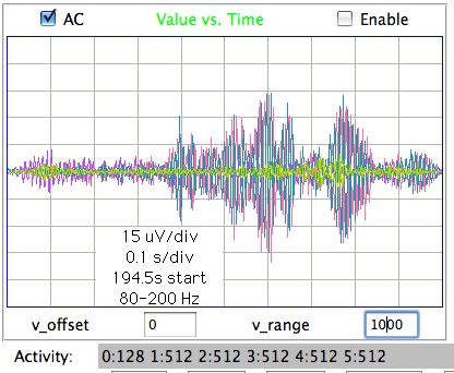
The impression one might get from the above plot is that there are 100 Hz oscillations in the signal. But here is the same signal band-pass filtered to 40-200 Hz.
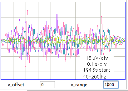
There are no 100 Hz oscillations. The signal contains oscillations of roughly 50 Hz. These vary in frequency during the one-second interval. These oscillations are asymmetric. In the Fourier transform, frequency variation and waveform asymmetry manifest themselves as frequency components at double the oscillation frequency. We call these double-frequency components the "second harmonics". The main, 50 Hz, components are the "fundamental frequencies" or "first harmonics". If you remove the first harmonics you are, of course, left with the second and higher harmonics. Here is the same EEG interval filtered to 120-200 Hz.

Here is a 64-Hz square wave we imported into the Neuroplayer. You can see the spectrum of the oscillation on the right, and on the left the oscillation itself in green. We plot the third harmonics on its own in purple. We extracted them with a 160-180 Hz band-pass filter.There is no second harmonic because the waveform is symmetric. But there is a third harmonic because the edges of the oscillation are sharp.
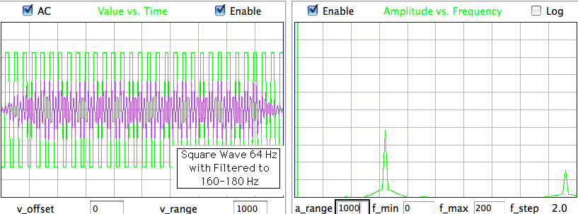
We cannot use bandpass filters to deduce the presence of oscillations at a particular frequency. By definition, a harmonic is not an oscillation. The oscillation is the sum of all the harmonics. These harmonics emerge when we transform the original signal into an abstract place called the "frequency domain". We are permitted to say that there are "oscillations at 100 Hz" only if there is no fundamental harmonic at 50 Hz.
[22-MAR-12] In Pitfalls of high-pass filtering for detection of epileptic oscillations, Clinical Neurophysiology, 2010, Benar et al. make the same argument we present above. In Continuous high-frequency activity in mesial temporal lobe structures, Epilepsia, 2012, Mari et al. apply an 80-Hz high-pass filter to epileptic human EEG and observe continuous high-frequency oscillations in the output of the filter. The examples below show how this will always be the case. We take one second of EEG from a non-epileptic, active mouse (recorded at Oxford University, 25-JUL-11, archive M1311606907, we picked 40-41 s at random) and apply three sharp high-pass filters: 40 Hz, 60 Hz, and 80 Hz. In each case, we see the apparent frequency of oscillation is about 20 Hz above the filter cut-off frequency.
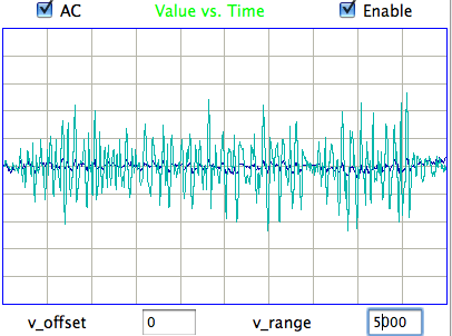
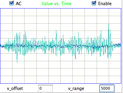
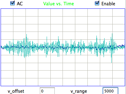
When we apply a step function to a filter, its output will ring afterwards, at a frequency close to the cut-off frequency. The ringing continues for longer as the filter gets sharper.
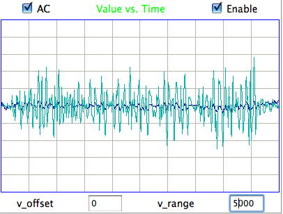
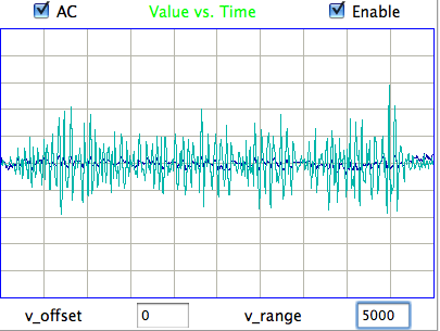
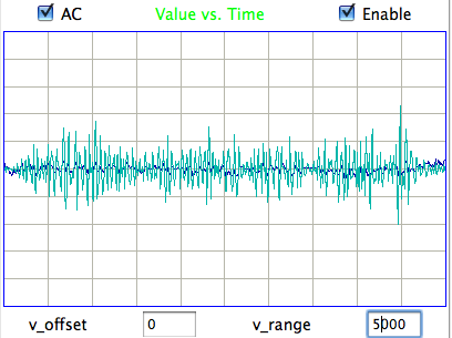
Filters with a more gentle cut-off produce ringing of smaller amplitude that decays more quickly. The images above show the same data we presented above, with the same cut-off frequencies, except that the high-pass filter allows a fraction of components less than 20 Hz below the cut-off frequency to remain in the filtered signal. The frequency response of the filter, in terms of amplitude, looks like a straight line from zero at 20 Hz below the cut-off, to one at the cut-off. Despite the gentle nature of this filter, we see that the same filter-generated oscillations remain in the signal.
[15-JAN-12] In the previous section we showed that the Fourier transform's amplitude spectrum alone was insufficient to identify high-frequency oscillations (HFOs) in EEG. In general, no matter what the appearance of the original signal, there will be other signals of dramatically different appearance with exactly the same amplitude spectrum. Their Fourier transforms are distinguished by the phases of their frequency components, not by the amplitudes. Thus the amplitude spectrum is not an adequate representation of the EEG signal for the identification of HFOs. In this section we present general-purpose definition of adequate representation that applies equally well to our Event Classifier and the Fourier spectrum.
Suppose we have an interval of EEG or some other signal, made up of M samples. Each sample xi has a one-dimensional value. In the case of the SCT system, the samples have integer values between 0 and 65535 as produced by the sixteen-bit analog to digital converters on the transmitters. We can think of each interval as being a point, x, in an M-dimensional space. Let S be the set of all possible intervals. In the case of the SCT system, S is an M-dimensional cube of side 65535 with one corner at the origin.
Let A ⊂ S represent the set of all intervals of a particular type. Thus A might represent the set of all intervals that contain one or more HFOs, or it might represent the set of all intervals that contain seizure spikes. For any interval x ∈ S, we can examine the interval ourselves and determine whether x is in A or not. In the SCT system, we would look at x as it appears in the voltage versus time plot of the Neuroplayer. Complimentary to A, we have a set S−A which contains all intervals that are not members of A. Obviously, A ∪ S−A = S and A ∪ S−A = ∅.
Our objective is to pick out from a large number of intervals those that are members of A. We can do this by eye, but it takes several seconds per interval, and if we have a million intervals, the task becomes impractical. Thus we set out to perform the classification with a computer. This we do by transforming each interval into another form, and classifying the interval based upon some simple proximity or threshold rules we apply to this other form. In general, we transform points in S into points in another space T. In Similarity of Events we transform 512 consecutive sixteen-bit samples into six real-valued metrics, each of which is a number between zero and one. Thus T is a six-dimensional unit cube with one corner at the origin. In Harmonics and Fundamentals we transform 512 consecutive sixteen-bit samples into 256 components of an amplitude spectrum. Thus T is a 256-dimensional cube with one corner at the origin. (The sides of this cube have length 65535 * √2, but that's not so obvious.)
Let F be a function such that for any x ∈ S we have y = F(x) is the transform of x, with y ∈ T. We call F our transform function. Furthermore, we write F(A) to represent the set of all points y ∈ T such that there exists x ∈ A for which y = F(x). Thus F(A) is the transformed version of A. In the same way, F(S−A) is the transformed version of S−A.
The discrete Fourier transform of an interval, including both amplitude and phase information, is a one-to-one transformation of points in the time domain, S, into points in the frequency domain, T. Given any point in T we can deduce the one and only point in S from which that point could arise. The function F is invertible, which is to say that F−1(y) exists, where F−1(F(x)) = x. If we use only the amplitude spectrum of the Fourier transform, however, the transformation is no longer one-to-one. The function F−1(y) does not exist, and for any y ∈ T there are many x ∈ S such that F(x) = y. When we transform intervals into six metrics, it is clear that we cannot deduce the original signal from the transformed point. What we can hope for, however, is that y = F(x) contains enough information for us to deduce whether or not x ∈ A.
By construction, we have A ∩ S−A = ∅ and A ∪ S−A = S. We don't care if F(A) ∪ F(S−A) = F(S) = T. Indeed, when we restrict S to a finite number of recorded intervals, we will find that F(S) is a proper subset of T. But we certainly prefer to have F(A) ∩ F(S−A) = ∅. If not, there exist points y ∈ F(A) ∩ F(S−A) such that y is the transform of at least one point in A and one point in S−A. In other words, we cannot use y to determine if x ∈ A. We say F is ambiguous with respect to A. The set of points x ∈ S such that F(x) ∈ F(A) ∩ F(S−A) is the ambiguous region of S with respect to A. The set F(A) ∩ F(S−A) is the ambiguous region of T with respect to A.
If we are to use F to determine if x ∈ A, the function must be unambiguous with respect to A. If F is invertible, then it will certainly be unambiguous with respect to A. But we want to work with functions that greatly reduce the amount of information our computer must deal with when applying our classification rules. In that case, F will not be invertible. We can, however, prove that F is unambiguous with respect to A by going through all members of S, inspecting each by eye, transforming them, and constructing the ambiguous region of S with respect to A. If this region is empty, then F is unambiguous with respect to A.
But in practice, S will contain too many members for us to inspect all of them. If S is the set of all possible combinations of 512 sixteen-bit samples, for example, it will contain 65536512 points. Even if we restrict S to the set of all such combinations that we have actually recorded from a laboratory animal, the number of points in S will still be too large, because our original motivation for applying F to S was that it would take too much effort to inspect each and every point in S. In practice, therefore, F will not be invertible and it will be impractical to classify all members of S by visual inspection. But the requirement that F be unambiguous with respect to A remains.
Thus we need a practical procedure to show that F is unambiguous with respect to A. To do this, we will assume that S contains a finite number of points. This will indeed be the case in practice, even if that finite number is tens of millions of seconds of recorded signal. We now place further conditions upon F. Loosely speaking, we require that F be such that we can define F(A) with a finite set of spheres. In more precise language, F must be such that there exists a finite set of points L ⊂ T and a radius r > 0 such that the union of all spheres of radius r centered on the members of L, which we will call U, is such that F(A) ⊂ U and F(S−A) ∩ U = ∅. When such an L and r exist, we say that F separates A, and that U provides an adequate representation of A in F. We see that F separates A implies that F is unambiguous with respect to A.
Our task, therefore, is to find an adequate representation of A in F, because if we can do that we show at once that F is unambiguous with respect to A and we know F can separate A from S−A. Given any x ∈ S, we check to see if F(x) ∈ U, where U is our adequate representation of A in F, and if so, we know x ∈ A, but if not, we know x ∈ S−A.
In certain cases, we may find that there are other ways to determine if F(x) ∈ U besides going through all the spheres of U and checking to see if it contains F(x). For example, if one of our metrics is high-frequency power and another is intermittency, we might say that x is an HFO if the high-frequency power, intermittency, and purity of the signal all exceed certain thresholds, or lie within certain bounds. But it could be that the threshold for high-frequency power should be a function of the intermittency, in which case our fixed-threshold classification would perform poorly. Even if constant thresholds could give us effective classification, we would still be left with the task of determining the values of the thresholds. Indeed, after many hours spend adjusting such thresholds, we concluded that classification with constant thresholds is impractical.
We are left with the task of composing a list of points, L ⊂ T, and choosing a radius, r, that together will provide us with an adequate representation of A in F. Consider the following separation algorithm.
If it is true that F separates A, this algorithm will eventually provide us with an adequate representation of A in F. If we find, after inspecting a sufficiently large number of points in S, that r has converged to some final value, and we are no longer adding points to L, we can be confident that we have an adequate representation. We will not be certain, but we can at least be confident.
In the case where A is a very small subset of S, such as when we are looking for rare features in a recorded signal, our algorithm is not efficient in its use of inspector time. It requires the inspector to examine a large number of uninteresting events. If possible, we should devise some simple criterion for initial rejection before inspection. The Event Classifier, for example, uses its first metric for initial rejection. If this metric is less than one half, the Event Classifier assumes that the interval is not an event (it assumes x ∉ A). Furthermore, the algorithm is inefficient in its use of the points in L because it allows them to extend influence only over a distance r. The Event Classifier overcomes this inefficiency by using a nearest-neighbor search through L to determine if F(x) ∈ F(A) or F(x) ∈ F(S−A). Thus the points in L have influence over all points in S to which they are nearest, and therefore all points in S are included in the sphere of influence of at least one member of L.
[18-JUL-25] We would like to detect wave packets of center-frequency 100-200 Hz in human EEG recordings. In the epilepsy community, these wave packets are called HFOs (high-frequency oscillations). Our sample EEG recordings are provided by Athena Lemesiou (Institute of Neurology, UCL). They come from intracranial electrodes implanted in the brains of adult patients with epilepsy. The recordings contain seizures, rumble, and mains hum. On some channels we see one or two HFOs per minute, but on others we see none. We would like to ignore the non-HFO features and extract from the signal the wave packets. At the same time, we are aware of how easily we can create wave packets by the action of high-pass filtering, as we discuss above. We resolve not to classify the EEG intervals by looking at a filtered version of the signal. We will look at the original signal.
Although we will not use filtering in our visual identification of HFOs, we will use the power in the 80-260 Hz band to pick out intervals that might be HFOs. These intervals will be our events and the 80-260 Hz band will be our event band. Our hope is that we can train a computer to classify events as HFO or non-HFO. The upper limit of 260 Hz makes no sense for signals recorded at 512 SPS, but in this case our EEG data was recorded at 1024 SPS and filtered to 268 Hz. The power of our HFOs should lie entirely within the event band. We will use event-band power for baseline calibration. Our event-power metric is a measure of the ratio of the event power to the baseline power. After some examination of the data, we set our event trigger at ten times the baseline power.
We found that symmetry and spikiness were not useful in detecting HFOs, neither when applied to the 80-260 Hz signal nor to the 10-40 Hz signal. But intermittency remains useful, this being the power of fluctuations in the de-modulated event-band signal. We devised a new metric to measure the purity of a wave packet. A wave packet has a gaussian-shaped frequency spectrum. Our purity metric is a measure of how narrow this peak is compared to its center frequency. A sustained sinusoid will have maximum purity and a spike will have minimum purity. A wave packet is somewhere in-between. Our ECP2 classification processor implements these three metrics. In the figure below we see a classification library arranged by purity and intermittency. The other two combinations of metrics give similar separation of HFO and Other events. All three metrics are necessary for adequate separation of the two classes.
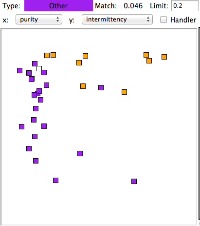
We built up our classification library by starting with channel No1 in an archive P9_HG_N4_REF_1.ndf for which ION had confirmed twelve HFOs. We used six of these in our library three others we found ourselves. We included twenty Other events from channel No1. We applied the library to all fourteen channels in the same archive. We found 5 New events and classified these. We applied the library again. We found 0 New events, 24 HFO, and 175 Other. Going through the 24 HFO events we find they all match our visual criteria. Our false positive rate among detected HFO events is less than 1/24 = 4%. Our false positive rate among randomly-selected 0.5-s intervals is less than 1/16800 = 0.006%. Going through the 175 Other events, we find seven or eight that we think should have been classified as HFO. These are either too close to the edge of the interval or accompanied by large artifacts that make detection difficult. Because we have roughly 32 HFO events and we miss 8 of them our false negative rate is 25%.
[23-NOV-18] The Batch Classifier generates lists of events, each of which is one playback interval long. With a one-second interval, a one-minute seizure may appear as sixty consecutive ictal events in an event list. Or the seizure might begin with four ictal events, and end with the first stretch of four non-ictal events. A feeding session could consist of five consecutive chewing events and end when we have ten consecutive non-chewing intervals. Making a list of such longer-term events, each of which consists of many interval-length events, is what we call event consolidation.
Our CEL4V1 program (Consolidate Event List V4.1) is a LWDAQ Toolmaker script. Open the Toolmaker in the Tool Menu, press Load, and select the script file. Press Execute. The following window opens.
We read an event list with the read_events button. A file browser window opens up. The event list should be one produced by the Batch Classifier. We let the program know the interval length used for event classification with the interval_length parameter, which has units seconds.
Our event list can contain events from any number of channels. The CEL4 selects events arising on one particular channel number we specify in channel_id. If we want to include events from two different channels in our consolidation, perhaps because we are using a dual-channel transmitter and an ictal event on either should count towards a seizure, we use an earlier version of the consolidator, CEL3V2, which uses all events in a list regardless of channel number. We have the Batch Classifier write a list of all events from the channels that we want to include, and apply CEL3V2 to this list.
The CEL4V1 and CEL3V2 consolidation algorithms begin by looking for a minimum number of consecutive events in the list. If we set min_start_intervals to 5, any sequence of five events in consecutive playback intervals marks the start of a consolidated event, and the start time will be the time of the first interval.
The consolidator's criterion for the termination of a consolidated event is the occurrence of more than a maximum number of break intervals during the consolidated event. If we set max_break_intervals to 4, then 5 consecutive playback intervals that do not contain an event will cause CEL2 to complete the current event, with the end of the consolidated event being the end of the final event it contains.
The event list written by the consolidator uses a ten-digit UNIX timestamp to mark the start time of the event, plus a fractional offset if such is necessary to get to the exact start time. Following the offset is the channel number of the first event in the consolidated event, its type, and the event duration. The name of the consolidated list we compose from the original event list, by adding a suffix, which you can specify with the consolidated_suffix parameter.
Example: We use Library_03FEB15 and ECP15V3 to produce a list of one-second ictal events in six separate hours of dentate gyrus field potential in a rat. We two hours before perforant pathway stimulation and several hours afterwards, not contiguous. We apply the consolidator, asking for five consecutive interval events to start a seizure and allowing no more than four break intervals. We obtain seven events in the recordings after stimulation and none in the recordings before. If we increase the minimum start events to ten, we get only one seizure, which is the one identified as the first seizure after stimulation by the group making the recordings (Philipps University, Marbug).
In the Neuroplayer, select the consolidated list in the Event Navigator. Step through the consolidated events to view them. Note that you can view the events with a longer playback interval than was used to obtain the original list of short events. If we use one-second intervals to make a list of ictal events, for example, we can view the consolidated events with 16-s intervals to see the evolution of a seizure on a longer timescale.
[19-MAY-17] Our new spike-finding algorithm SCPP4V1 is not fooled by the kind of step-changes in EEG that are generated by the movement of imperfectly-secured electrodes.x We plot our EEG signal as a sequence of points on a two-dimensional map. The grid squares of the map are one sample period wide. For a 512 SPS signal, the map squares are 1/512 s wide. The squares are one mean absolute step size high, where the mean absolute step size is the one-dimensional coastline of the signal divided by the number of samples. For baseline mouse EEG recorded with a skull screw, the map squares will be roughly 15 μV high.
We move along the EEG path in discrete steps. Each step moves us to a later point in the EEG signal. We try to make the step as small as possible. If we can take a smaller step by skipping one or more points, we do so. Points that we skip represent abberations from the path traced by the EEG signal. Our measure of the size of an aberration is the greatest distance from the aberration to the point we step to. We see the path-tracing in action below.
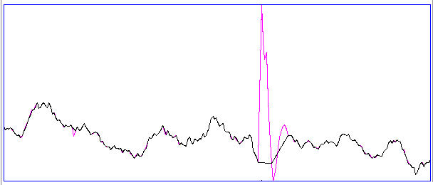
When the size of the aberration is greater than our spike_threshold, we classify the aberration as a spike. The threshold has units of mean absolute step size. A threshold of 20 works well to find spikes in transgenic mouse EEG. In the figure below we see how a step-artifact does not generate a spike detection with the path-finding algorithm.
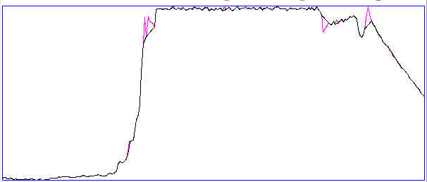
We enhance the spike-finding by limiting the number of points we are permitted to skip when taking a step along the path. This number is the spike_extent. An extent of ten forces the path-tracer to follow any aberration that is more than ten samples long. Inter-ictal spikes recorded in mice at 512 SPS are less than ten samples long, but electrode artifact spikes are more than ten samples long. The M1445359478 archive, from University of Edinburgh, is notable for its 30-mV movement artifacts in channel No5 as well as a variety of smaller movement artifacts. To test how well we can find spikes in all manner of intervals, we inserted an artificial 700-μV spike in our data as we went through archive M1445359478 in 8-s intervals.
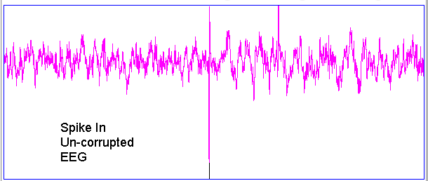
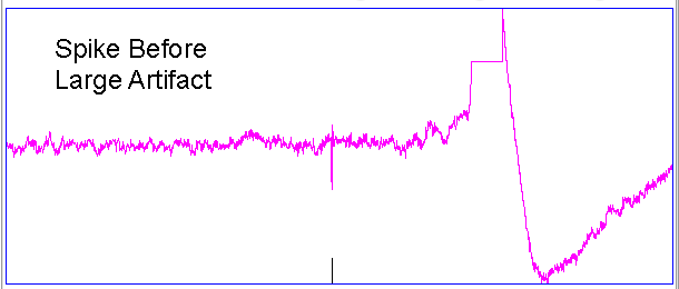
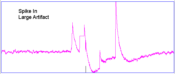
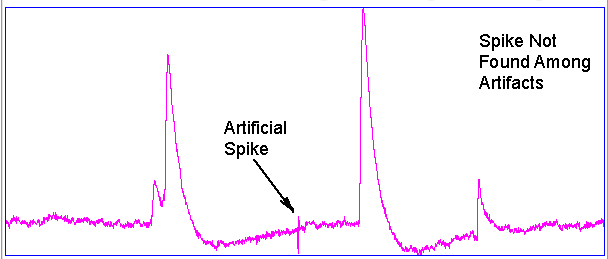
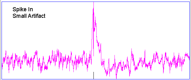
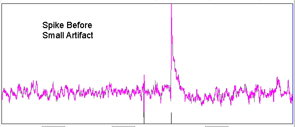
Out of 450 intervals in the M1445359478 archive, there are only one interval in which we do not find the artificial spike. In this interval, which we show in the figure above, huge artifacts have so greatly increased the mean absolute step size that the spike does not exceed our threshold. Our false negative rate on this archive is 1/450.
We use the SCPP4V1 processor to measure delta power (0.1-3.9 Hz) and count spikes in each 8-s interval of M1445359478. We sort the intervals in order of decreasing delta power. All intervals with delta power >100 ksqcnt (90 μV rms) contain some kind of movement artifact. We look at all these intervals and count false spikes, which are all caused by edges and features on artifacts, and actual spikes among the artifacts. We do this same experiment for spike thresholds 10 and 20. Considering the 27 intervals with delta power >100 ksqcnt, there are no obvious inter-ictal spikes we miss with either threshold 10 or 20.
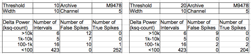
We repeat this experiment with M1436545502 channel No6, in which the largest movement artifact is only a few millivolts, but their leading edges are sharp. We see artifacts generating false spikes as in this interval. We summarize the performance of the spike finder in the following two tables for thresholds 10 and 20.
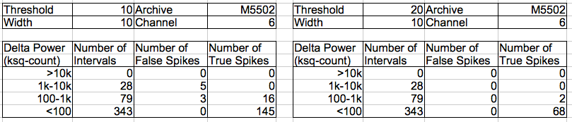
A threshold of 20 detects half as many spikes as a threshold of 10. But the threshold of 10 increases our false spike count from zero to eight. Considering the 145 intervals with delta power >100 ksqcnt, there are 3 obvious inter-ictal spikes we miss with threshold 20 and none we miss with threshold 10.
When spikes come in tightly-packed clusters of three or more, we want to count them as bursts rather than spikes. The figure below shows separate spikes occurring in the same interval, and a sequence of spikes that are part of a single burst.
To distinguish spikes from bursts, and to count both features, SCPP4V1 first obtains a list of small spikes. It goes through this list of small spikes and finds large solitary spikes to count as spike features and closely-packed clusters of spikes to count as burst features. The output of SCPP4V1 for the three-spike interval above looks like this:
M1459881430.ndf 2488.0 2 0.0 3.0 0.0 37.123 62.882
We have the archive name and the time of the interval start. The interval is 8 s long, but this value is not recorded in the characteristics line. The signal is channel number 2. The signal loss is 0.0%. The interval contains 3 spikes and 0 bursts. The delta and theta power are 37 and 63 ksqcnt respectively, or 54 and 71 μV rms. (See above for conversion between ksqcnt and μV rms.)
[15-JUL-25] Here we present event classification using the generation-twenty event classification processor, ECP20, which has been in use since 2018 and has attained a comfortable level of stability. For a history of event classification and the evolution of its classification processors, see our event classification appendix, where we break up the evolution into chapters, each chapter covering the performance of a new classification processor. For a complete inventory of classification processors, see their code directory.
The ECP20 event classification processor provides six dimensionless, bounded classification metrics for each playback interval. Each of these is a sigmoidal function of some underlying classification measurement. The metrics are bounded from zero to one, but the measurements can have any other real-valued range. The ECP20 processor is designed to operate with one-second intervals, so each second of a signal will be characterised by six metrics, and each metric is itself a number. The metrics are power, coastline, intermittency, coherence, asymmetry, and spikiness. They are "dimensionless" because they are normalized. In the case of the power metric, the normalization is with respect to a reference power value specified somewhere in the processor script. In the case of the other five metrics, they are self-normalizing with respect to each interval. The metrics are "bounded" because their values are constrained to lie in the range zero to one. We use ECP20 with the Neuroplayer's Event Classifier to classify intervals of EEG for the purpose of event detection. The ECP20V4R1 metrics are optimized for 1-s intervals of 160 Hz, 512 SPS EEG recordings and 1-s intervals of 80 Hz, 256 SPS EEG recordings. The processor detects the signal sample rate and adjusts its metrics accordingly.
In addition to metric calculation, ECP20 provides an event handler that allows us to detect and respond to events in live recordings or count events in existing recordings. We invite you to download our ECP20 Demonstration Package (290 MBytes), which contains ECP20V2, EEG recordings, and an event library that you can try out with the Event Classifier. The ECP20 processor does not use the Fourier transform. It executes at the same speed as ECP16. The only difference between ECP20 and its predecessor ECP19 is that ECP20 has dropped the rhythm metric, added event handling code, and supports 80-Hz, 256 SPS EEG as well as the original 160-Hz, 512 SPS EEG. Here is how the ECP20 script declares the names of the metrics.
set config(classifier_metrics) "power\
	coastline\
	intermittency\
	coherence\
	asymmetry\
	spikiness"
To each classification metric, we first calculate a classification measurement. Both the measurements and the metrics are dimensionless, real-valued measurements of some property of the signal. The measurements can cover any range of values, but the metrics are bounded from zero to one. In ECP20, we obtain the classification measurements with metric calculation "E", which we call with lwdaq_metrics command. The processor will print out details of the classification measurements when we set metric_diagnostics to 1. In the paragraphs below, we provide a detailed description of each classification measurement.
Power: The power measurement is the standard deviation of the interval divided by the baseline standard deviation, as specified in the Neuroplayer's calibration panel. When we transform this measurement into the power metric with a sigmoidal function. The interval and baseline standard deviations are both expressed in units of sixteen-bit sample counts, or cnt. When the interval amplitude is equal to the baseline amplitude, the power metric is 0.5. We recommend you do not use the power metric for event detection. Doing so requires that you pick baseline values for each pair of electrodes, or assume that each pair of electrodes has the same sensitivity to EEG. Your study will be simpler and more robust if you use only the normalized metrics that follow.
Coastline: The coastline measurement is the sum of the absolute changes in signal value from one sample to the next, divided by the number of samples in the interval, divided by the range of the signal in the interval. The range of the signal is its maximum value minus its minimum value. If the range is zero, we set the coastline measurement to zero also. A typical value of coastline measurement for baseline EEG is 0.07.
Intermittency: The intermittency measurement is the fraction of the coastline generated by the 10% largest absolute sample-to-sample changes in signal value. We call the movement from one sample to then next a step. The absolute sample-to-sample change is the absolute value of the difference between the first and second sample values when we take one step through the signal. We make a list of all the absolute changes, sort them in descending order, and take the first 10% of them. We add them up to obtain the coastline generated by the 10% largest steps. We divide this coastline by the total coastline to obtain our intermittency measurement. A typical value of intermittency measurement for baseline EEG is 0.27, for ictal EEG is 0.36, and for grooming artifact is around 0.5. Small changes in the measurement represent large changes in the nature of the signal.
Coherence: The coherence measurement is the fraction of the normalized display area occupied by the ten biggest peaks and valleys. For each peak-valley pair, we calculate the area of the smallest rectangle that encloses the peak and valley. This area is the change in signal value multiplied by the change in sample number. If we were to convert the signal value into voltage, and the sample number into time, the area would have units Volt-second. We add the ten largest areas and divide by the total area of the display to obtain our coherence measure. The total area of the display is the range of the signal multiplied by the number of samples in the interval. We adjust the coherence calculation with the coherence threshold, which we multiply by the signal range to obtain a minimum height for peaks and valleys. Smaller peaks and valleys we ignore. In ECP20 the default value of the threshold is zero, so all peaks and valleys are added to our list. If your signal is noisy, you can try increasing the coherence threshold to 0.01 or even 0.02 to ignore noise and focus on larger movements of the signal. The coherence metric is the most effective metric for separating ictal activity from baseline signal in EEG. The coherence measurement of one-second intervals of baseline EEG varies from 0.02 to 0.06, while that of ictal activity varies from 0.08 to 0.16. The coherence measurement is the only metric that behaves differently as we increase the interval length. For two-second intervals, the coherence measurement will be half as large, because we are using only ten peaks and valleys in our calculation. If we want to use the coherence metric with longer intervals, and obtain the same values of the metric for longer intervals filled with the same activity, we do so by modifying the sigmoidal function that converts the coherence metric from the coherence measurement.
Asymmetry: To obtain our asymmetry measurement, we take the absolute value of the third moment of the signal, which is the sum of the third power of each sample's deviation from the mean. We divide this absolute value by the third power of the standard deviation of the signal to obtain our asymmetry measure. A typical value of asymmetry measurement for one-second intervals of baseline EEG is 0.2, and for an inter-ictal spike is 4. Note that the mesurement, and the subsequent metric derived from the measurement, is insensitive to the direction of the asymmetry.
Spikiness: To obtain our spikiness measurement, we divide the interval into overlapping sections and measure the range of the signal in each section. The spikiness measurement is the ratio of the maximum section range to the median section range. This measurement is sensitive to sharp steps up and down as well as to solitary spikes. In the ECP20 event classifier, we specify spikiness extent in units of samples. The width of each section is two extents plus one. The sections are separated by one extent, so they overlap. With an extent of 2, each section is 5 samples wide, and the sections are spaced by 2 samples. In a 512 SPS signal, 5 samples is 10 ms, so we will be most sensitive to spikes with edges that are less than 10-ms in duration. A typical value of spikiness measurement for one-second intervals of baseline EEG is 3, and for an inter-ictal spike is 20.
The classification metrics are increasing functions of the classification measurements, with minimum value zero and maximum value unity. We transform the classification measurement into the classification metric with the following sigmoidal function.
Here M is the classification metric, A is the classification measurement, C is a measurement center value, and s is a sensitivity. The metric has value one half when the measurement is equal to the measurement center value. On either side of the center value, the sigmoidal function approaches zero or one more rapidly with increasing sensitivity. The ECP20V4R1 processor's sigmoidal functions are optimized for use with 160-Hz and 80-Hz bandwidth EEG recordings. The differences in the sigmoidal functions for these two sample rates are minor, with the exception of the spikiness sigmoidal function. The 160-Hz spikiness center is twice the 80-Hz spikiness center. Both processors are optimised for 1-s intervals.
One of the tasks of a classification processor is to declare event types and colors for use in the Event and Batch Classifiers. Each study requires its own list of event types, depending upon what the study is looking for, and the native language of the researchers. Nevertheless, the ECP20 script provides the following types and colors by default.
set config(classifier_types) "Ictal red \
	Hiss blue \
	Depression cyan \
	Spike orange \
	Grooming darkgreen \
	Artifact lightgreen \
	Baseline gray"
We will be using these types and colors in our examples. By Spike we mean a solitary pulse in the interval. Spike events are most often inter-ictal activity. By Ictal we mean an interval that looks like an epileptic seizure, with coherent pulses and asymmetric waves. By Hiss we mean intermittent or sustained high-frequency activity more powerful than baseline. By Depression we mean periods of quiet after a seizure, where the signal is far less powerful than baseline, and contains very little low-frequency activity. By Grooming we mean bursts of high-frequency EMG that have crept into the EEG recording through exposed electrode surfaces. By Artifact we mean large steps generated by insecure electrodes and spikes generated by signal corruption. And by Baseline we mean normal EEG.
To illustrate the ECP20 metrics, we take as an exercise twenty hours of recordings from two healthy mice, and three hours from two mice injected with pilocarpine. Electrodes are bare wires held in place with screws and covered with dental cement. We process all recordings with ECP20 and generate characteristics files that contain the ECP20 metrics for one-second intervals. From the three epileptic hours we obtain confirmed and obvious ictal events (sample). From the entire twenty-three hours, we obtain obvious examples of spikes (sample), grooming (sample), and baseline (sample) events. All events are one-second intervals. The result is Library12JUN19KH, which we we invite you to use as a starting point for a new study. Load the library into the Event Classifier, and select the ECP20 processor in the Neuroplayer.
In the map of intermittency versus coherence, we see robust separation of ictal intervals from all other types. Grooming and spike events are close to one another, but they are distinct from baseline events. If our objective is to find only ictal events, we can do so with onl the intermittency and coherence metrics. But if we want to separate grooming from spike events, we need another metric. The map below shows the coastline metric separating grooming and spike events.
The grooming event with the lowest coastline (see here) is close to the spike event with the highest coastline (see here). But the intermittency of this grooming event is high, placing it far from the spike events in the intermittency versus coherence map. We enable only coastline, intermittency, and coherence in the Batch Classifier, set the match limit to 0.2 and make a list of spikes in the twenty hours recorded from healthy mice. Of 158201 intervals, 483 contain signal loss (99.7% reception), and 1628 are classified as spikes. When we hop through the list, however, we find that half the spikes are in fact grooming artifact.
When we examine the map of spikiness versus coastline, it does not appear that spikiness will be of any help separating grooming from spikes. But when we look at the map of spikiness versus intermittency, we see that these two metrics are, on their own, able to separate spikes from grooming.
With the spikiness, coastline, intermittency, and coherence metrics enabled, we repeat the same batch classification and get a list of 883 spikes, of which nine out of ten are best described as spike events. The following map illustrates the asymmetry metric. The asymmetry metric is good at distinguishing between grooming artifact (sample and sample) and spikes (sample).
The table below presents measurements of the total time taken to play the same sixty-second archive containing sixteen signal channels of various sample rates. We turn on and off the plots and the Fourier transform calculation. We turn on and off the processor. We always run the propcessor with the Quiet box checked, so as to disable writing lines of test to the Neuroplayer text window.
We vary the number of 512 SPS channels we process by means of the Neuroplayer's channel select string. We measure how long it takes to play our sixty-second sample archive. The ECP20 processor itself takes roughly 2 ms per 512 SPS channel per second of recording. Most of the playback time is consumed by signal reconstruction. We also vary the playback interval length, to see how this affects processing time. But the ECP20V2 and ECP20V3 processors remain optimised for 1-s intervals.
[15-JUL-25] By "closed loop control" we mean event classification followed by a stimulus based upon the results of classification. In addition to metric calculation all version of the ECP20 processor, such as ECP20V2, define an event handler that detects seizures in real-time by classifying each EEG interval as it is received, and looking for a certain number of consecutive ictal or spike intervals before deciding that a seizure has begun. In the ECP20V4R1 processor, the handler responds to a seizure by sending a command to an Octal Data Receiver (A3027) that causes one of its digital outputs to change state and provoke some stimulus, such as turning on a lamp for optogenetic suppression of a seizure. Newer versions of ECP20 direct an A3042B Telemetry Control Boxes (TCBs) to issue a command to an Implantable Stimulator-Transponder (IST) to flash an implanted Fiber-Coupled LED.
The ECP20 event handler supports any number of channels simultaneously. The handler allows us to randomize our response to seizures by assigning a probability to the response, and it allows us to turn on and off the stimulus during a set seizure response period. See the handler-defining code at the end of ECP20V4R1 for more details.
To illustrate closed-loop control, we apply ECP20V2R2 to fourteen hours of EEG recorded from four mice with A3028B transmitters. The four mice are channel numbers 17, 21, 23, and 25. All four are epileptic. Once we have all fourteen characteristics files, we load Library02JUL19KH into the Event Classifier and enable the coastline, coherence, asymmetry, and spikiness metrics. We set the power threshold to zero so that we are classifying only on the appearance of the signal, not its amplitude. We set the match limit to 0.1. In the Batch Classifier we select all fourteen characteristics files as input, specify text file Ictal_Spike.txt as output, select ictal and spike events for detection, list our four transmitter numbers, and press Batch Classify. We find 198k intervals with good reception, and 3k with poor reception. The Batch Classifier ignores those with poor reception. Of the 198k with good reception, 3407 are classified as ictal or spike. These events are stored in Ictal_Spike.txt. We select Ictal_Spike.txt with the Neuroplayer's Event Navigator and hop at random through the list of events, assessing visually the actual type of each event. Of 100 events we examine, we believe 92 are indeed ictal or spike. Our false positive risk among 3407 detected ictal and spike events is 8%. Among the 198k intervals without loss, our false positive rate is 0.14%. In an attempt to determine the false negative rate for ictal and spike detection, we search for all event types other than ictal and spike, including events of type Unknown. We get 195k such events. We examine 200 of these and fine 2 that we think are ictal or spike, and these are classified as Unknown. This suggests that there are 1900 ictal and spike events that are being ignored by our classification, so our false negative rate is roughly 36%, and our sensitivity is 64%.
We repeat our experiment, but this time with match limit 0.05. Our new list of ictal and spike events contains 704 entries. Of 100 events we examined visually, we believe all 100 are either ictal nor spike. Our false positive rate is now close to zero among detected events, and vanishingly small among all intervals. But our previous experiment suggests that there are 4300 ictal and spike events, so our false negative rate is now 86%.
We activate the ECP20 seizure-detector by checking the Handler box in the Event Classifier. As soon as we read and display one interval of EEG from our NDF archive, the handler window, shown above, will open. The handler illustrates what is possible with the Event Classifier when applied to live seizure detection, and to off-line event counting. The handler waits for trig_len consecutive ictal or spike intervals on any one of its selected channels. When it encounters such a sequence, it initiates a seizure response that lasts for en_len intervals. With match limit 0.1, our false positive rate for ictal and spike detection is 0.14%. According to our calculation above, a trigger length of three intervals should be proof against a trigger being generated by false positives alone. A trigger length of five intervals will make it less likely that we trigger on short period of inter-ictal activity.
The handler allows for us to initiate the stimulus at random once the seizure is detected. The probability that the stimulus response will be applied is en_prob. If the stimulus is applied, it will be switched on for on_len intervals and off for off_len intervals repeatedly until en_len intervals have passed. If the stimulus is not applied, no stimulus commands will be sent, but the handler will wait for en_len intervals before it starts looking for another trig_len sequence of ictal or spike intervals. The IP address and LWDAQ Driver socket values come from the Receiver Instrument. The Enable checkbox enables TCPIP activity. Uncheck this box to make lists of seizures off-line. The IP and Socket entries give the IP address and socket of a LWDAQ device that will initiate the stimulus. Most likely, this device will be an Octal Data Receiver. The On and Off parameters are the commands we send to an Octal Data Receiver to generate a stimulus. Future versions of the handler will support commands being sent to a Command Transmitter to instruct implanted stimulators.
The channels to which the event handler will apply seizure-detection are listed in the handler window. They are the same channel numbers listed in the Neuroplayer's channel select string at the time the handler window was first opened. List the channels you want to analyze in this select string, close the event handler window, and play one EEG interval to re-create the handler window with your list of channels.
The seizure-detector writes enable on and enable off times to an event list on disk. The name of the event list is in the Outfile entry box. This file is one you browse with the Neuroplayer's event navigator. The enable-on times are the last interval of the trigger sequence. The enable-off times are the last interval of the response. The Verbose option turns on additional text messages.
We apply the seizure-detector to four fourteen hours of EEG from four epileptic mice, with trig_len set to 3. We get a list of 110 seizures. We go through these and find that all of them are initiated with ictal and spike activity. Some are long and some are short, but none are what we would call a false positive.
[12-MAY-25] We have moved much of the historical content of this page to an Appendix.
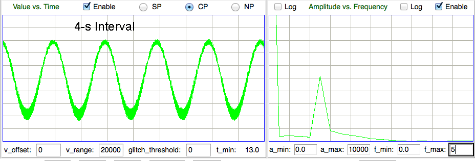
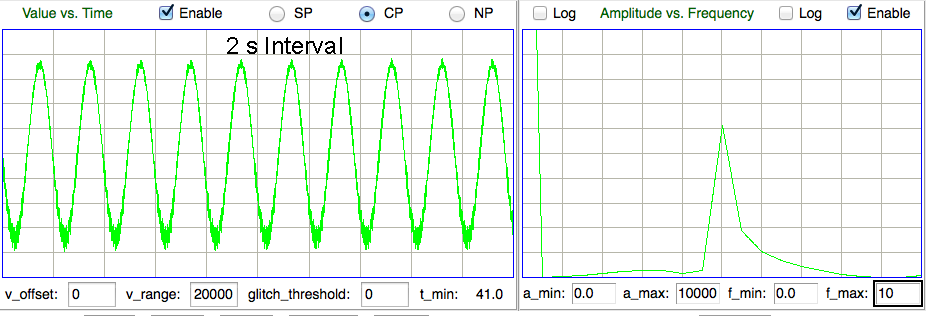
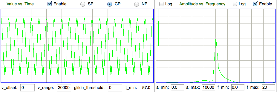
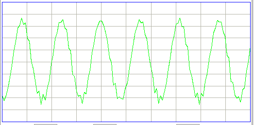
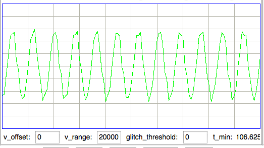
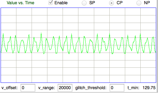
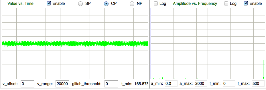
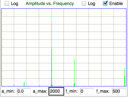
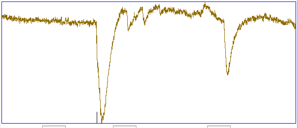