[12-MAY-25] Here we present appendices to our Event Detection manual. We present the history of event classification processors, starting with the earliest. We begin with ECP11, which classifies short EEG events that occupy a significant portion of the playback interval, and does so without calculating the Fourier transform of the signal. The calculation is fast and robust. The ECP11 was our first successful, fast processor, and we studied its performance in detail. We preserve that study in the paragraphs below. We improved upon the glitch filter and the metric calculations in ECP15 and ECP16, which we describe in their own sections. The ECP18 processor introduced a metric that detects arbitrarily short spikes in a long interval, as well as re-introducing the Fourier transform to measure theta and delta power.
Our descriptions of event classification processors are backed up by demonstration archives that we make available on our Example Recordings page. There you will find demonstration archives for the EXP3, ECP11, ECP19, and ECP20 processors. We offer further examples of the application of our classification processors in the Development Appendix.
[22-DEC-14] Here we present our ECP11, and describe how to use it to perform calibration and event detection. This work is Stage Two of our Analysis Programming collaboration with the Institute of Neurology, UCL. Download the latest LWDAQ from here. Download a zip archive containing recordings, characteristics files, event library, processor, and example event list by clicking here (370 MBytes).
The ECP11 processor calculates six metrics: power, coastline, intermittency, spikiness, asymmetry, and periodicity. All are either entirely new, or calculated in a new way that enhances their performance. We will describe each in turn. We will introduce normalized classification and normalized plots, and show how the improved metrics, combined with normalized classification, provide us with a new solution to the calibration problem. The ECP11 metrics are not calculated in the TclTk script of the processor. They are calculated in compiled Pascal code. You will find this code in metrics.pas, in the eeg_seizure_A procedure. Pascal is easy to read, and we have added comments to explain each step of the calculation. Because the metrics are calculated in compiled code, execution time is greatly reduced.
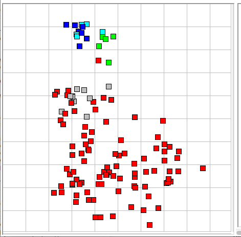
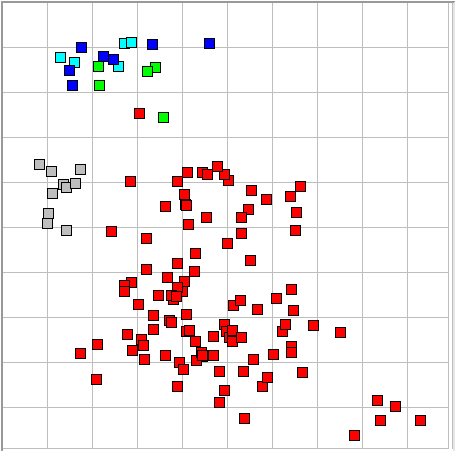
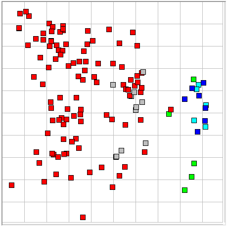
Consider one-second intervals of EEG recorded from the motor cortex or visual cortex of an epileptic rat. We want to detect intervals containing solitary spikes, trains of spikes, sustained oscillations, or combinations of all three. Our purpose is to find ictal and inter-ictal activity. At this stage, we will not attempt to distinguish between the various forms of such activity. Any interval activity we deem to be ictal or inter-ictal, we will call ictal. Ictal events will be red squares in our classifier maps. Ictal events are powerful compared to the baseline signal. An artifact is a powerful event generated by some source other than EEG. It might be a transient caused by a loose electrode, a bursts of EMG introduced into the EEG while the animal is chewing, two transmitters using the same channel number, or a step change in voltage caused by a disturbance of one of the electrodes. Artifacts will be green squares in our maps. A hiss event is EEG activity dominated by sustained 60-120 Hz activity. (Such a spectrum is called "hiss" in electronics, after the sound that gives rise to the same spectrum in audio circuits.) Hiss events will be dark blue squares.
We have two event types that are less powerful than ictal, artifact, or hiss. A baseline interval is one showing an approximate pink-noise spectrum, with no obvious oscillations, spikes, or bursts, but at the same time having the rumble as we expect in the EEG of a healthy animal. A baseline event will be a gray square in our maps. A depression is an interval with very low power, no rumble, and a spectrum similar to that of white noise. A depression will be a light blue square. There are two other types that always come with the Event Classifier: normal is any event with power metric less than the classification threshold, and unknown is any event with power metric greater than the threshold, but lying farther than the match limit from any event in the classification library. A normal event is white and an unknown event, if we happen to have one by mistake in our library, is black.
The first metric we calculate for event classification is the power metric. It is also, by long-standing tradition, the first metric we record in the characteristics of each interval for classification. Because our subcutaneous transmitters have capacitively-coupled inputs, the average value of the digitized signal bears no relation to the power of the biological signal. We begin our power measurement by subtracting the average value of each interval, and consider only deviations from the average as indications of signal power.
As a measurement of the amount of deviation during the interval, we could use the mean absolute deviation, the standard deviation, or the mean square deviation. We will calculate our power metric by applying a sigmoidal function to our measure of deviation, and this sigmoidal function raises the deviation to some power that gives us good separation of events in our event map. The standard deviation and the mean square are equivalent for our purposes. But the mean absolute deviation is distinct from the standard deviation. Within an interval, the standard deviation gives four times the weight to a point twice as far from the average while the mean absolute deviation gives only twice the weight to the same point. Because we are looking for events that contain spikes, we would like to promote the contribution of larger deviations in the signal make to our power measurement. Thus we choose the standard deviation of the signal as our measure of power, and denote this P.
In previous processors, we chose a frequency band in which to calculate power. In ECP1, we took the Discrete Fourier Transform (DFT), selected all components in the range 1-160 Hz and used their sum of squares as our power measurement. Before we calculate the DFT, however, we must apply a window function to the first and last 10% of the interval. The window function makes sure that the first and final values are equal to the average. The DFT is the list of sinusoids that, when added together, generates an exact replica of the interval, repeating infinitely. In the case of one-second intervals, the sum of the DFT sinusoids produces a replica of the original interval that is exactly correct at the sample points, and repeats every second. Any difference in the first and final values of the interval appears as a step between these repetitions, which would require many high-frequency sinusoidal components to construct, even though there is no evidence of such components in the original one-second interval.
The window function, however, will attenuate any interesting features near the edges of the interval. If there is a spike near the edge, the window function will taper it to zero. This tapering will make is smaller and sharper at the same time. We will see less overall power than is present in the original signal, but more high-frequency power. If there is a low-frequency maximum at one end of the interval, the window function will turn it into something looking more like a spike. Baseline EEG can be distorted by the window function into something similar to ictal EEG, which greatly hinders our efforts to distinguish between baseline intervals and the far less numerous ictal events.
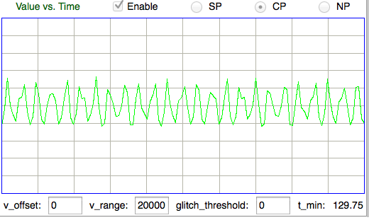
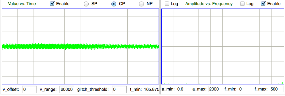
For these reasons, the ECP11 processor makes no use of the DFT whatsoever, neither in calculation of the power metric nor any other metric. In order to accelerate processing, the script disables the calculation of the DFT in the Neuroplayer by setting the af_calculate parameter to zero. The Neuroplayer will calculate the DFT only if we enable the amplitude versus frequency plot in main window.
We do, however, apply a glitch filter to the signal before we calculate its power. Glitches are artifacts of faulty radio-frequency reception. We remove them by going through the interval and finding any samples that jump by more than a glitch threshold from their neighbors (for latest implementation of the glitch filter, see here). We apply the glitch filter before we plot the signal in the VT display, so the signal we see is the same as the one from which we are obtaining the power measurement. For this study, we set the glitch threshold to 2000, which means any jumps of 800 μV from one sample to the next will be removed as glitches.
To obtain our power metric, P_m, we apply the glitch filter and calculate the standard deviation of the result, which we denote P. We transform P into a metric between zero and one with the following sigmoidal function.
P_m = 1 / (1 + (P/P_b)−1.0)
Where P_b is our baseline power calibration for the recording channel. In this study, we assume a default value of 200.0 counts for P_b, which means the power metric will be one half when the signal's standard deviation is two hundred counts. In an A3019D or A3028E transmitter, two hundred of our sixteen-bit counts is an amplitude of 80 μV. In our experience, baseline EEG in healthy rats is 20-50 μV, so we expect the power metric of our baseline intervals to be between 0.2 and 0.3. We note that the metric has greatest slope with respect to interval power when the signal amplitude is 200.0 counts rms.
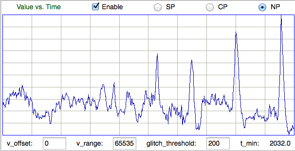
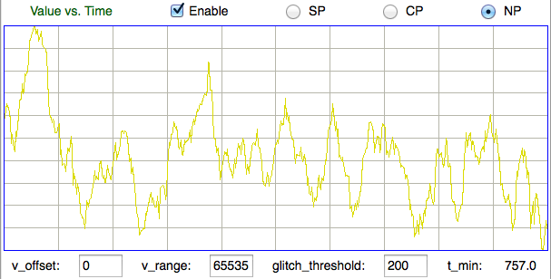
The power metric is the only one of our six metrics that depends upon the amplitude of the signal. The remaining five are normalized with respect to amplitude. Their values are dependent only upon the shape of the signal during the interval. A normalized plot of the interval signal, in which the signal is scaled to fit exactly into the height of the display, helps us see the shape of the signal independent of its amplitude. The Neuroplayer provides a normalized plot of the signal with the NP button above the VT display. If the normalized metrics perform well, any two intervals with a similar appearance in the normalized plot of the signal will be close to one another in the classifier's metric space. If we want to see the absolute power of the signal in the VT plot, we use the CP mode to get a centered display with a fixed height, or SP mode to get a display with fixed height and offset. These two display modes were previously implemented with the AC button, which could be checked or unchecked.
Ictal activity has higher amplitude than normal EEG. Our calibration of an EEG recording is an effort to find the amplitude above which an interval is likely to be ictal, and below which it is unlikely to be ictal. We use this amplitude as a threshold for classification. Any interval above above the threshold is a candidate event, and any below, we ignore.
The Event Classifier provides a classification threshold. We set its value in the classifier window. An event with power metric greater than or equal to the classification threshold is a candidate event. All other intervals are normal. The Event Classifier and the Batch Classifier apply this threshold when classifying events from all channels. If we analyze one channel at a time, we can calibrate each channel by entering a different value for the classification threshold. We want a value that is greater than the power metric of most baseline intervals, but less than the power metric of almost all ictal intervals. If we set the classification threshold to zero, all intervals will be classified, which we call universal classification.
If ictal intervals are rare, we can use the power metric's ninety-ninth percentile point as our classification threshold. If the minimum amplitude we see in an hour-long recording is an indication of our baseline amplitude, we could use a multiple of this baseline as our classification threshold. In ION's recent recordings, however, there are hours in which ictal intervals outnumber baseline intervals, and hours in which depression intervals reduce the minimum interval amplitude by an order of magnitude compared to our imagined baseline. We can use neither a percentile point nor a minimum amplitude. Nor can we divide the maximum amplitude by some factor to obtain our threshold, because an hour in which we have no ictal events would have a threshold that was too low, and an hour in which we had several large, transient artifacts would have a threshold that was too high.
If we permit ourselves to examine the signal by eye and set the threshold using our own judgment, we could, through confirmation bias, end up lowering the threshold for control animals, and raising it for test animals, so as to create a difference in the ictal event rate when no such difference exists. Aside from saving us time, automatic event detection is supposed to avoid human bias in the counting of EEG events. Whatever system we have for determining the amplitude threshold, it must be objective.
The Event Classifier and Batch Classifier permit us to refrain from using any particular metric by un-checking its enable box along the bottom of their respective windows. When we disable the power metric for classification, the power metric is still compared to the classification threshold to determine if the interval is worthy of classification, but once an interval's power metric has exceeded this threshold, the power metric will not be used again. The classification will be based only upon the metrics that are enabled. If we set the classification threshold to zero as well as disabling the power metric, every interval will be classified using the normalized metrics alone.
The five normalized metrics produced by ECP11 are able to distinguish between ictal, baseline, and depression intervals most of the time. This ability allows us to count baseline intervals and calibrate each recording channel using the following procedure. We set all baseline power values to 200 in the Calibration Panel. We apply the ECP11 processor to the recordings we want to calibrate, processing all channels at once, and recording characteristics to disk. We load our event library into the Event Classifier, for example Library_20DEC14. The library must contain a selection of baseline events. We open the Batch Classifier. We select our ECP11 characteristics files as input. We select the channel we want to calibrate. We disable the power metric. We set the classification threshold to 0.0. We apply batch classification and obtain a count of the number of baseline intervals detected by normalized classification for threshold = 0.0. We do the same for increasing values of classification threshold. We are looking for the threshold value that causes a sudden drop in the number of baseline events. The figure below shows how the number of baseline events varies with classification threshold for the eight active channels in archive M1363785592.
For the eight channels in M1363785592, a classification threshold of 0.40 eliminates roughly 99% all baseline events, and a value of 0.35 eliminates roughly 90%. Aside from comparing an interval's power metric to the threshold, we will not use the power of the signal for classification. We will classify intervals above threshold using only the five normalized metrics. This comparison confuses baseline intervals with ictal intervals less than 1% of the time. Our threshold already rejects 99% of baseline intervals, so we will get fewer than one false ictal classification per hour. With a threshold of 0.35, we get a few false ical events per hour.
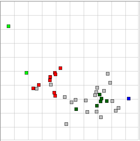
Now we must consider how many ictal events will be ignored because they fall below the classification threshold. The power versus periodicity display of our event library shows that a few of our ictal events fall just below 0.40 in their power metric. (Power is the horizontal axis from zero to one.) A threshold of 0.35 will accept almost all ictal events, while a threshold of 0.40 will overlook of order 5% of them. In our experiments, we used a threshold of 0.40, but we may in the end find that 0.35 is a better choice. In any case: the threshold we choose based upon the graphs above is the calibration of our recording.
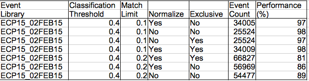
The table below shows how the number of ictal, baseline, and depression events in sixteen hours of recordings from epileptic animals is affected by threshold, match limit, normalization, and exclusive classification. Exclusive classification is where we ignore events in the event library that are not of one of the types selected in the Batch Classifier. The match limit is the maximum distance from a library event for an interval to be considered to have the same type.
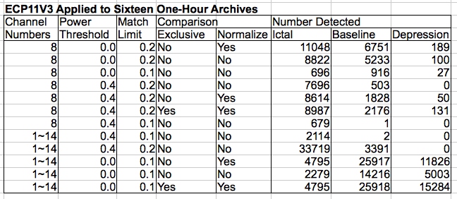
Of interest in the table above is the identification of depression events. These have power metric 0.1-0.2. When we set the classification threshold to 0.0, the match limit to 0.2, and use normalized classification on channel 8 only, we get a list of 189 depression events. Of these, many are actually far more powerful hiss events. The depression event is similar in appearance to a hiss event, but with lower amplitude.
The periodicity metric is a measure of how strong a periodic or oscillatory component is present in an interval. In metrics.pas we go through the signal from left to right looking for significant maxima and minima. By significant we mean of a height or depth that is comparable to the mean absolute deviation of the signal, rather than small local maxima and minima. The ECP11 processor has a show_periodicity parameter that, if set to 1, will mark the locations of the maxima with red vertical lines, and the minima with black vertical lines. The figure below shows a normalized plot of an ictal event with the maxima and minima.
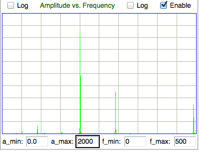
If we take the DFT of the same interval, we see a distinct peak at 12 Hz. But the DFT does not have a distinct peak for the following interval, even though it is obviously periodic and ictal. The periodicity metric, however, detects the periodic component of the interval.
The periodicity calculation produces an estimate of the period of the oscillation in the interval, but this estimate does not appear in the metric. In the future, we expect to use this estimate to track changes in the oscillation frequency of a developing seizure. For now, we use the metric only to measure the strength of the periodic component. In the following interval, the calculation detects some periodicity.
The periodicity metric almost always detects the presence of a periodic component that is visible to our own eyes. But the periodicity detection sometimes it fails, as in the following example.
The above interval is, however, sufficiently powerful and intermittent to be classified as ictal, even if its periodicity is not detected. We may be able to improve the periodicity calculation in future so as to detect the periodicity in this interval, but as the calculation stands now, making it more sensitive to periodicity compromises its rejection of random noise in the far more numerous baseline intervals.
Depression and hiss events also have low periodicity. The figure below shows a depression event.
In order to reduce the chances of random noise appearing as periodicity, we pass through the signal from left to right locating maxima and minima, and then from right to left doing the same thing. We get two values of periodicity. We pick the lowest value. If the signal has a genuine periodic component, both values will be close to the same. If it is the result of chance, the probability of both values being high is less than one in ten thousand.
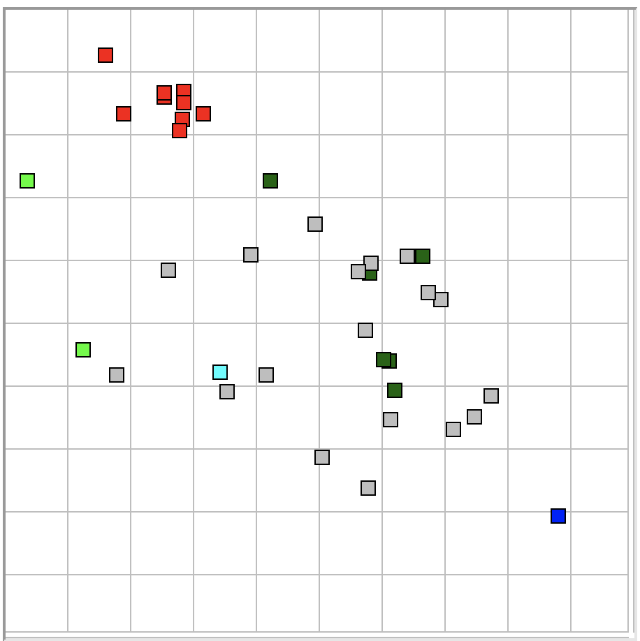
The figure above shows our event library map with the power metric as the horizontal axis and periodicity as the vertical. We see that only ictal events have high periodicity.
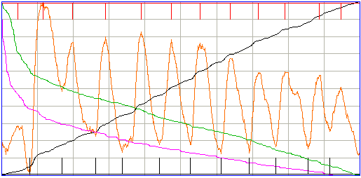
The coastline of the interval is the sum of the absolute changes in signal value from one sample to the next. We divide the coastline by the mean absolute deviation of the signal to obtain a normalized measure of how much the signal shape contains fluctuation. Periodic ictal events have low coastline, because they achieve high absolute deviation without changing direction between their maxima and minima. Depression events have high coastline because all their power consists of small, rapid, fluctuations. Hiss events have high coastline for the same reason.
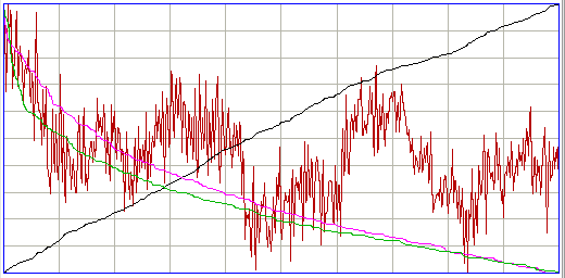
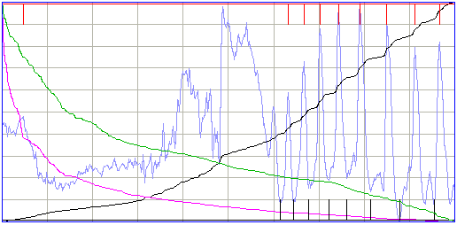
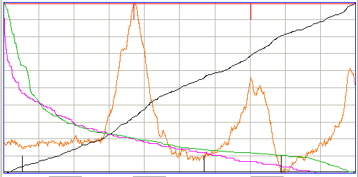
The black line in the above plot shows how the coastline is increasing as we move from left to right. The line starts from zero and ends at the total coastline for the entire interval. In the following artifact interval, we see the coastline climbing in steps as bursts of high frequency activity occur.
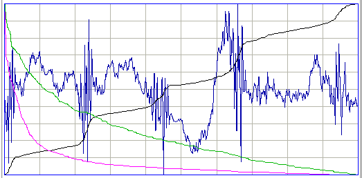
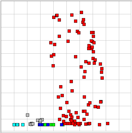
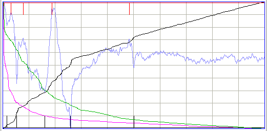
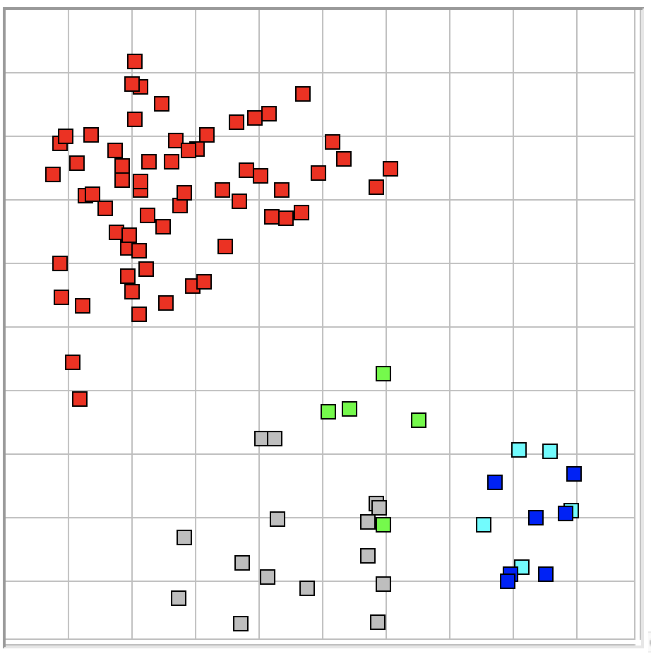
The intermittency metric is a measure of how concentrated the coastline is in segments of the interval. We sort the samples in order of decreasing absolute change from the previous sample. The purple line is the graph of absolute change versus sample number after we perform the sort. We calculate the coastline accounted for by the first 20% of sorted samples and divide by the total coastline to obtain a measure of intermittency. We pass this through a sigmoidal function to obtain the intermittency metric. The figure below shows how coastline and intermittency, both normalized metrics, separate ictal and baseline events from all other types of event.
In this map, we see that baseline events have low intermittency, but so do some ictal events. The ictal events with low intermittency, however, almost all have high periodicity or spikiness, and so may still be distinguished from baseline.
Aside: Our ECP1 classifier provided a high frequency power metric in place of our coastline. We divided the DFT power in 60-160 Hz by the power in 1-160 Hz. This worked well enough, but could be fooled by the action of the DFT's window function upon large, slow features at the edges of the interval. The coastline metric is far more robust and does not require a DFT. The ECP1 provided intermittency also, by taking the inverse transform of the 60-160 Hz DFT components, rectifying, taking the DFT again, and summing the power of the 4-16 Hz components. The two additional DFT calculations made this a slow metric to obtain, and it was still vulnerable to the window function artifact. Our new intermittency metric is more robust, easier to illustrate with one purple line, and a hundred times faster.
The ECP1 classifier provided spikiness and asymmetry, but the calculation in ECP11 is more robust. The following ictal interval is powerful, spiky, but symmetric.
This interval is powerful, spiky, and asymmetric.
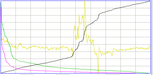
To detect spikiness and asymmetry, we sort the samples in order of decreasing absolute deviation from the mean. The green line in the plot above, and indeed all our interval plots, shows the absolute deviation versus sorted sample number, scaled to fit the height of the display. We add the absolute deviation of the first 20% of the sorted samples and divide by the total absolute deviation to obtain a normalized measure of spikiness, for this shows us how much the interval's deviation is concentrated in segments of time. We apply a sigmoidal function and so obtain the spikiness metric.
To measure asymmetry, we take the same list, sorted in descending order of absolute deviation. We extract the first 20% of samples from this list, and select from these the ones that have positive deviation. We add their deviations together and divide by the sum of the absolute deviations for the same 20%. We see that a result of 1.0 means the entire 20% largest deviations are positive, and 0.0 means they were all negative. We apply a sigmoidal function to obtain our asymmetry metric.

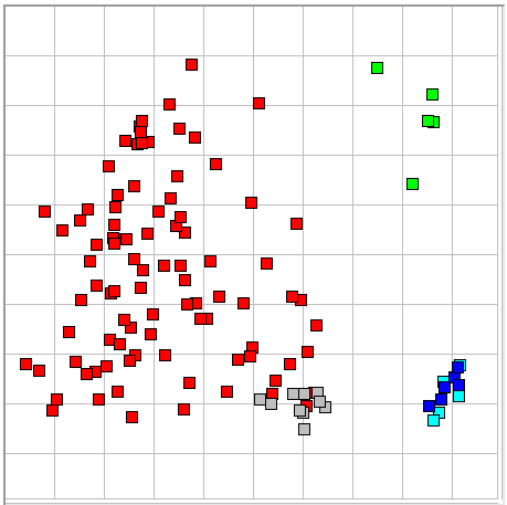
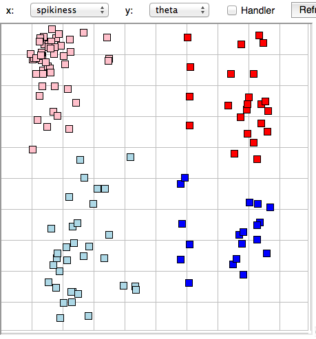
The figure below shows how our library events are distributed by spikiness and asymmetry in the classifier map.
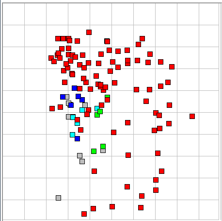
Only ictal events have high spikiness, and most asymmetric events are ictal. But there are plenty of ictal events mixed in with the other types in this map. The asymmetry metric is not particularly useful in distinguishing between baseline and ictal events. But it is useful in distinguishing between different forms of ictal event, and so we retain the asymmetry metric for future use in seizure analysis.
The following table breaks down the time taken to process each second of each channel of recording at 512 SPS by Neuroarchiver 97, LWDAQ 8.2.9, and ECP11V3 on a MacOS 2.4 GHz Dual-Core machine.
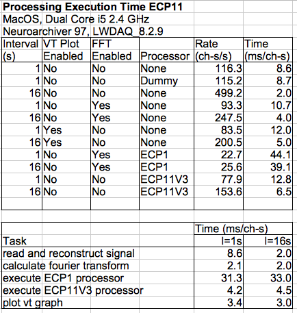
The ECP1 processor takes 31 ms to process a 1-s interval, but it requires the Neuroplayer to execute its Fast Fourier Transform (FFT) routine, so the total metric calculation time for ECP1 is 33.3 ms/ch-s. The ECP11 processor does not use the FFT. Its total execution time is 4.2 ms. We disables the plots and the FFT in two instances of LWDAQ on our dual-core machine, and attained an average rate of 130 ch-s/s. The new processor is eight times faster than ECP1, its metrics are more robust, and the additional periodicity metric allow far more reliable separation of baseline and ictal intervals.
[23-DEC-14] We apply Batch Classification to our sixteen hours of example recordings to create a list of ictal events. We open the list in the Neuroplayer. The list is usually thousands of events long. We jump around at random within the list and count how many events out of one hundred are, in our opinion, ictal. This fraction is our measure of the classification performance. We repeat this experiment with different event lists and classifier configurations. The following table summarizes our observations.
Aside: The Hop button to take a random jump within an event list so as to facilitate the measurement of classification performance.
Detail:There was one ictal event in the 19DEC14 library that was causing many incorrect normalized matches with baseline intervals. We removed this event and added a new hiss event to create the 20DEC14 library.
[24-DEC-14] Our sixteen hours of recordings contain 230k channel-seconds of EEG. With threshold 0.40, match limit 0.10, and normalized classification, we find 3065 ictal events. Of these, roughly 122 are mistakes, which gives us a false ictal rate of 0.05%. If we raise the match limit to 0.2, we find 32486 ictal events, of which roughly 2900 are mistakes. We have found ten times as many ictal events, but our false ictal rate has jumped by a factor of thirty.
We examine the mistaken ictal events. Half of them are powerful baseline events that are almost, but not quite, ictal. Often, these events are preceded and followed by ictal events. Sometimes they are not. In either case, the mistaken identity is not the result of artifact. The remainder are artifacts not generated by EEG. In particular, there is an hour recorded from a transmitter No3 in which there are many large transients, and another hour in which many ictal-like events are caused by two No13 transmitters running at the same time.
With threshold 0.40 and match limit 0.20, the normalized and un-normalized classification produce the same ictal count and the same false ictal rate.
If we eliminate the No3 transients and the No13 dual-recording, and accept that almost-ictal events will sometimes be mistaken for ictal, the remaining mistakes are the ones that will remain with us and confuse our analysis. These mistakes occur at a rate of roughly 0.1%, or several per hour. If several mistakes per hour is too high to tolerate in our study, we can try reducing the match limit to 0.10.
Our 20DEC14 library contains 119 reference events. Most of them are ictal. Their distribution with coastline and intermittency, or spikiness and coastline, shows us that many events are farther than 0.1 metric units away from their neighbors. In our five-dimensional normalized metric space, many ictal events have no neighbor closer than 0.3 metric units away. Their distribution with power and periodicity in our six-dimensional un-normalized space shows open spaces 0.2 units wide. If we want to find all ictal events using a match limit of only 0.1, we must add ictal events to our library to fill the empty spaces in the ictal volume. Assuming a random distribution of events in a connected n-dimensional volume, reducing the average separation between the events by a factor of two requires 2n times more events. In our five-dimensional normalized space, we will need roughly four thousand events, and in our six-dimensional un-normalized space, eight thousand.
Increasing the library size will slow down batch processing, but batch processing is not a large part of our total analysis time, so it may indeed be practical to use an event library containing thousands of events. But we would rather work with a library of a hundred events. With some more work on the calculation of the periodicity metric, and perhaps the elimination of the asymmetry metric, we are hopeful that we can reduce the false itcal rate to an acceptable level with such a library.
[02-FEB-15] The ECP15 classification processor is an enhanced version of ECP11. We presented ECP15 to ION, UCL with a talk entitled Automatic Seizure Detection. The talk provides examples of half a dozen event types, displayed in the Neuroplayer with metric calculations marks.
The ECP15 processor generates up to six metrics: power, coastline, intermittency, spikiness, asymmetry, and periodicity. It produces an estimate of the fundamental frequency of the interval, which it expresses as the number of periods present in the interval. The power, coastline, and intermittency metrics are calculated in the same way as in ECP11, as described above. But the spikiness, asymmetry, and periodicity metrics have been enhanced so as to provide better handling of a large population of random baseline intervals. To calculate metrics, ECP15 uses eeg_seizure_B, a routine defined with detailed comments in metrics.pas, part of the compiled source code for the LWDAQ 8.2.10+ analysis library. An event library for use with ION's visual cortex recordings is Library_02FEB15.
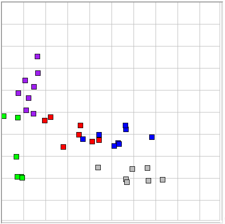
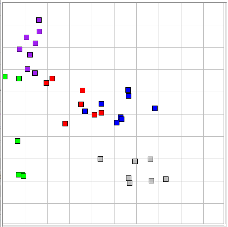
When we look at the arrangement of event types in the coastline versus intermittency map, we see that we have adequate separation of most ictal events (red) from the baseline examples (gray). But there are some ictal events overlapping baseline events. We present two examples below.
The ictal interval is periodic, slightly asymmetric in the upward direction, and contains large, smooth-sided, sharp spikes. The baseline interval is not at all periodic, slightly asymmetric in the downward direction, and contains two large excursions that are neither clean nor sharp. Among the other ictal events in the baseline region of the coastline versus intermittency map, all contain sharp spikes, but the spikes can have rough slopes and they can have no fixed period.
The ECP15 spikiness calculation begins with a list of peaks and valleys. In the processor script, we enter a value for spikiness_threshold, which the minimum height of a peak or valley, expressed as a fraction of the signal range. If we use the signal standard deviation or mean absolute deviation, occasional intervals with a small number of sharp spikes will not be assigned a high spikiness, and will remain indistinguishable from baseline intervals.
In ECP15V3 we have spikiness_threshold = 0.1, so any peak or valley with height 10% the range of the signal will be included in the peak and valley list, and marked with a black vertical line when we have show_spikiness = 1. The spikiness measure is the average absolute change in signal value from peak to valley in units of signal range. This measure is bounded from zero to one, but we pass it through a sigmoidal function to provide better separation of points. The result is a coastline versus spikiness map as shown below.
There is one ictal event (red) near an artifact event (green). When we examine these two, we find that the artifact has high intermittency, and the ictal event does not.
In ECP15 we measure asymmetry by taking the ratio (maximum-average) / (average-minimum) for the signal values in the interval. A symmetric interval will produce a ratio 1.0. We pass this ratio through a sigmoidal function to obtain a metric bounded between 0 and 1. This calculation is simpler than the one we defined for ECP11, but it turns out to be far more reliable when applied to a large number of baseline intervals, and so we prefer it. We obtain a map of coastline versus asymmetry as shown below.
The asymmetry metric does not improve separation of ictal and baseline events. But it does allow us to distinguish between upward, symmetric, and downward ictal events. At the moment, we are bunching together spindles, spikes, spike trains, and all other remarkable activity under the type "ictal". When we want to distinguish between spindles and spike trains, the asymmetry metric will be necessary.
Our periodicity calculation is similar to that of ECP11. We obtain a list of peaks and valleys in the same way we do for spikiness, but using a separate threshold, the periodicity_threshold. In ECP15V3, this threshold is 0.3. We want only the largest peaks and valleys to be included in the list. The left-hand interval below is one with high periodicity. We turn on display of the long black marks with show_periodicity = 1.
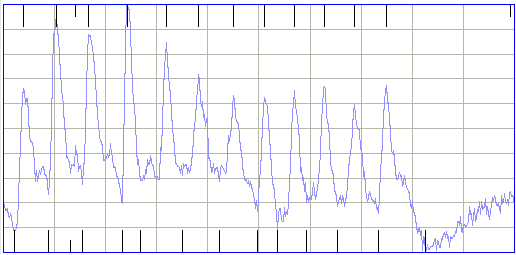
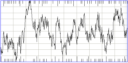
If there are many more spikiness peaks and valleys than periodicity peaks and valleys, we reduce the periodicity measure, because such a discrepancy is a feature of baseline intervals that produce periodicity at randome. The right-hand interval above is an example of one that would, at random, have high periodicity, but because of this reduction has lower periodicity. As a result of this additional precaution, the ECP15 periodicity metric remains less than 0.3 for almost all baseline intervals. Periodicity is low for most ictal intervals also, so the metric does not improve separation of ictal and baseline intervals.
The ECP15 periodicity calculation produces a best estimate of the fundamental period of the signal. Meanwhile, the periodicity metric is an indication of the reliability of this best estimate of period. With show_frequency = 1, ECP15 draws a vertical line on the amplitude versus frequency plot of the Neuroplayer window. The location of the line marks the frequency of the peaks and valleys in the signal, and the height of the line, from 0% to 100% of the full height of the plot, indicates the periodicity metric from 0 to 1. Thus the height is an indication of the confidence we have in the frequency. This combination of confidence and frequency allows us to monitor the evolution of oscillation frequency in long seizures.
The table below gives the processing time per channel-second of 512 SPS data for increasing playback interval. The processor is calculating all six metrics, even though we do not include the asymmetry and periodicity metrics in our characteristics files. We have all diagnostic and show options turned off in the ECP15 script.

The spikiness and periodicity metrics of ECP15 are more efficient than those of ECP11. On our laptop, with a 1-s playback interval, ECP15 takes 1.8 ms/ch/s to compute metrics, while ECP11 takes 4.2 ms/ch/s. The result is a 19% drop in the overall processing time for 1-s intervals. The ECP15 processing rate is 4.2 times faster than ECP1 for 1-s intervals, and 11 times faster than ECP1 for 16-s intervals.
We repeat the performance tests we describe above, but this time applying ECP15 to our data. There are 236887 channel-seconds in the sixteen hours of recordings.
In ECP15, we have reduced the number of metrics from six to four. The events in our library are more closely packed in the metric space. With match limit 0.1, we pick up as many events as we did with limit 0.2 when using six metrics in ECP11. Roughly 3% of the events identified as ictal are not ictal. Of these, most are two-transmitter artifact or faulty transmitter artifact, but we also have baseline swings, small glitches, and a few baseline events that fool the classification. With normalized, non-exclusive classification, we obtain 34k events with match limit 0.1 and 57k events with 0.2. Of the former, roughly 33k are correct, and of the latter, roughly 49k. By using a match limit of 0.1, we are missing at least one in three ictal events because our event library does not fill the ictal region in the metric space adequately. There are 240k intervals in all, and of these roughly 190k of these are not ictal. With match limit 0.1 we interpret 1k of these as ictal, making our false positive rate 0.5%.
[06-FEB-15] We apply ECP15V3 to recordings from the dentate gyrus provided by Philipps University, Marburg, during their initial six months of work, before they had set up their faraday enclosures. We use the same spikiness threshold. We have a different event library made up of events from these recordings, Library_03FEB16. Baseline power is 500 for all channels. There are 37 archives in all, containing 1M channel-seconds of recording. Of these, 910k have reception greater than 80%. The others receive power metric zero.
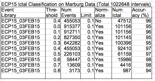
Even with threshold zero, using normalized classification, performance is 95%. Of 910k intervals, only 5k were classified incorrectly as ictal even without any use of the signal power. At threshold 0.4, we have 50% fewer events above threshold, but the number of classified ictal events drops by only 8%.
There are several hours of recordings during perforant path stimulation, and so we see in the recordings the pulses caused by the stimulation. These are often classified as ictal, and so we do not count them as errors, but they explain why there are so many events above threshold 0.8. Of the events above threshold 0.8, many are due to stimulation, and some are large baseline swings that we believe to be artifact, but are not ictal.
We instruct the Batch Classifier to find baseline events. We use threshold 0.4, match limit 0.1, and normalized classification. It finds two hundred thousand baseline intervals. We examine one hundred of these intervals and judge that 80% of them are baseline and 20% of them are ictal.
Combining these observations for threshold 0.4 and match limit 0.1, it appears that the chance of a baseline interval being mis-classified as ictal is around 0.5%. The chance of missing an ictal event is around 30%. If a seizure contains four consecutive seconds of ictal activity, the chance of missing the seizure is less than 1%. The chance of four seconds of baseline being classified as a four-second seizure are small, so that we expect no false seizures even in one million seconds of data.
[07-APR-15] With the release of Neuroarchiver Version 99, we can select which available metrics we want to use for event detection in the Event Classifier. The ECP16 processor produces six metrics: power, coastline, intermittency, coherence, asymmetry, and rhythm. It calls lwdaq_metrics with option C to obtain measures of power, coastline, intermittency, coherence, asymmetry, and rhythm. See our heavily-commented Pascal source code for details of the eeg_seizure_C routine in metrics.pas. Each measure has value greater than zero, but can be greater than one. These measures can provide event detection in a wide range of applications, provided we can disable some of them in some cases, and provided we can tailor the way the measures are transformed into their metric values. At the end of ECP16 processor script, we pass each measure to a sigmoidal function, along with its own center and exponent values. The center value is the value of the measure for which the metric will be one half. The larger the exponent, the more sensitive the metric value is to changes in the measure about the center value.

In the example above, we use intermittency center 0.4 to cluster the ictal events near the center, and exponent 4.0 to keep the intermittency metric away from the top and bottom edges of the plot. If we apply the same center and exponent to another experiment, we see the plot below on the left.
We would like to see better separation of the gray baseline events from the more interesting red and blue ictal events. We change the exponent value in ECP16 from 4 to 6 and the center from 0.4 to 0.35and obtain the plot on the right, which gives better separation.
The power and intermittency metrics of ECP16 are identical to those of ECP15, with the exception of the variability offered by ECP16's center and exponent parameters. The coherence replaces the spikiness metric, but is calculated in the same way. (The name "spikiness" had become misleading, because the metric was in fact a measure of how self-organized the interval was, rather than random, which is not well-described by the word "spikiness".) The rhythm metric replaces the periodicity metric, but is calculated in the same way. (The name "periodicity" suggested that the period of an oscillation was represented by the metric, but in fact it is only the strength of a periodic function that is represented by the metric.)
The ECP16 coastline metric is significantly different from ECP15 because we use the range of the signal rather than the mean absolute deviation to normalize the metric. The ECP16 processor has a far better glitch filter, so we are more confident of removing glitches before processing. We can use the range of the signal as a way to normalize the interval measures. The coastline metric in ECP16 is now normalized with respect to interval range, which means the coastline corresponds more naturally with what we see in the normalized Neuroplayer display.
The asymmetry metric in ECP16 is very much improved. The plot below shows separation of spindle and seizure events in Evans rats.

The asymmetry measure is 1.0 when there are as many points far above the average as below. In the plot above, the measure is 0.7 at the center of the display. Even spindles, it turns out, are biased towards negative deviation. But seizures are more so.
In addition to the six metrics, ECP16 counts glitches in the Neuroplayer's glitch_count parameter, and it will draw the dominant frequency of the interval on the spectrum plot in the Neuroplayer window.
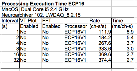
The table above shows processing speed with ECP16V1 and Neuroarchiver 102.
[22-SEP-16] The ECP18V2 processor introduces a spikiness metric that finds short, solitary spikes within an EEG interval.
Consider the above spike. In its eight-second interval, it has no significant effect upon any of the other metrics. In the spikiness calculation, we divide the interval into slices. Each slice is ten samples wide. In this case, ten samples is 20 ms, and there are 400 slices across the interval. We measure the range of the signal in each slice, and sort the slices in order of decreasing range. The spikiness measure is the ratio of the largest range to the median range. In ECP18V2 we set the spikiness metric to 0.5 when the spikiness measure is 7.0. With the show_spikiness parameter we can trace the upper and lower limits of the slices with two black lines, and plot the ranges with a separate purple line.
Also in ECP18V2 is a theta metric, which represents the ratio of the power in the theta band, which we define as 4-12 Hz, to power in the reference band, which we define as 0.1-3.9 Hz. In order to obtain the theta measure, we must calculate the frequency spectrum. The processor enables calculation of the Fourier transform for this purpose. As a result, the processor is slower than ECP16. With 8-s intervals, ECP!8V1 runs at 52 ch-s/s while ECP16V1 runs at 330 ch-s/s.
We use the spikiness and theta metrics to classify 8-s intervals into one of four types: theta without spike, theta with spike, non-theta without spike, and non-theta with spike. The following event library we arrived at in collaboration with Edinburgh University using EEG recorded from mice.
We later found that we wanted to examine both delta-band power and theta-band power, as well as count the number of spikes in each 8-s interval, for which we use the Spike Counter and Power Processor, SCCP1V2.tcl. If you want to use the spikiness metric, but you do not need the theta metric, edit ECP18V2 so as to remove the theta metric calculation and the enabling of the spectrum, so as to be left with an efficient classification processor.
[23-FEB-18] The ECP19V1 processor provides seven metrics: power, coastline, intermittency, coherence, asymmetry, rhythm, and spikiness. Each metric is a value between zero and one that acts as a measure of the property of the image after which the metric is names. To obtain the metrics, we first obtain positive-valued measure of the property, then we apply a sigmoidal function to the measure to produce a metric that spans almost the full range zero to one when calculated on our event library. In the paragraphs below, we describe how we calculate the measures from which we obtain the metrics. The actual calculations you will find in metrics.pas in the code defining the function metric_calculation_D.
Download a zip archive containing recordings, characteristics files, event library, processor, and example event list by clicking ECP19 Demonstration (730 MBytes, thanks to ION/UCL for making these recordings available). The power, coastline, intermittency, and rhythm metrics are identical to those of ECP16. The spikiness metric is identical to that of ECP18. The coherence and asymmetry metrics are new.
Power: Divide the standard deviation of the interval by the signal's baseline power. The baseline power is defined in the Neuroplayer's calibration panel. The ECP19 processor does not implement any form of adaptive baseline power measurement, but instead leaves it to the user to define the baseline power for each signal. We recommend using the same baseline power for all signals generated by the same part of the body, with the same type of electrode, and the same amplifier gain. For example, all mouse EEG recorded with an M0.5 skull screw using an A3028B transmitter could have baseline power 200 ADC counts.
Coastline: The normalized mean absolute step size of the interval. We sum the absolute changes in signal value from one sample to the next, then divide by the number of samples in the interval, then divide by the range of the signal during the interval.
Intermittency: The fraction of the coastline generated by the 10% largest coastline steps.
Coherence: The fraction of the normalized display occupied by the ten biggest peaks and valleys. The normalized display has the signal scaled and offset to fit exactly within the height of the display. We control this calculation with the coherence threshold. We multiply the coherence threshold by the range of the signal within the interval to obtain a height in ADC counts. This height is the minium distance the signal must descend from a maximum in order for the maximum to be counted as a "peak", and it is the minimum distance the signal must ascend from a minimum in order for the minimum to be counted as a "valley". Each peak is given a "score", which is the area of the smallest rectangle that encloses the peak itself and the valley that precedes the peak. If there is no such valley, the peak score is zero. The score, being an area in the normalized display, has units of count-periods, where the period is the time between samples. For a 512 SPS recording, the period is 1.95 ms. We score the valleys in the same way. We put the peaks and valleys together into a single list. We sort this list by score. We add the ten highest scores and divide the sum by the total area of the display to obtain the fraction of the display occupied by the largest peaks and valleys.
The default value of the coherence threshold is 0.01, as defined in the ECP19V1 script. If we decrease the threshold to 0.005, the coherence calculation will insist upon smoother lines to define peaks and valleys. If we increase the threshold, the coherence metric will tolerate more noise superimposed upon the peaks and valleys. In our experience, the optimal value can be anywhere from 0.001 to 0.02, and in some cases the adjustment of threshold is essential for adequate discrimination between baseline and ictal intervals. (Our "peak and valley" list is similar to the "turns" list used in EMG analysis as described by Finsterer.)
Asymmetry: We take the third moment of the signal, which is the sum of the third power of each sample's deviations from the mean, and divide by the standard deviation to obtain a value that is negative for downwardly biased intervals and positive for upwardly-biased intervals. We raise the natural number to this value to obtain a measure that is greater than zero.
Rhythm: The number of large peaks and valleys that are separated by roughly the same length of time, divided by the total number of large peaks and valleys. When we say "roughly the same length of time" we mean within ±20% of some value of "rhythm period". The calculation attempts to find a value of rhythm period that maximizes the rhythm measure. The routine returns not only the rhythm measure, but also the inverse of the rhythm period, which we call the "rhythm frequency". The rhythm threshold we pass to the metric calculation is similar to the coherence threshold in the way it defines the peaks and valleys. The rhythm threshold is the fraction of the signal range that a signal must descend from a maximum or ascend from a minimum in order for the maximum to be counted as a large peak or the minimum to be counted as a large valley.
Spikiness: We divide the interval into sections, each of width equal to the spikiness extent parameter we pass into the metric calculator. The spikiness extent is in units of sample periods. In each of these sections, we measure the range of the signal. We make a list of the section ranges and sort it in decreasing order. The spikiness is the ratio of the maximum section range to the median section range. This metric is sensitive to sharp steps up and down as well as spikes.
Consider the following one-second intervals of EEG. Both are recorded with A3028E transmitters implanted in rats at the University of Capetown. One contains large, coherent pulses, the other does not.
We would like to identify and count intervals with such pulses, but we are unable to do so with the ECP16 processor: it assigns the same coherence metric to both intervals, and similar values for coastline and intermittency. The ECP19 processor, however, can separate the above intervals with coherence alone. The following figure compares coherence in ECP16 and ECP19 using a library of events taken from the Capetown, which you can download as Lib28MAR17JR.
We use ECP19 and Lib28MAR17JR to count intervals with pulses in thirty-six hours of EEG recorded from several different rats at the University of Capetown. We obtain a list of 2300 intervals. We hop through 100 members of the list and find that 95 of them match our visual criteria for coherent pulses. The following figure compares coherence in ECP16 and ECP19 using the library of events we include in our ECP19 Demonstration package.

The ECP19 processor calls the lwdaq metrics routine with version "D", from which it obtains eight real numbers, including a frequency value associated with the rhythm metric. The ECP19 processor does not use the Fourier transform of the signal, and so proceeds at roughly the same speed as ECP16. We processed 600 of 1-s intervals with 14 channels of 512 SPS each on a MacOS i5 2.5 GHz machine with both the VT plot and the FFT calculation disabled. Processing with ECP16 took 92 s and with ECP19 took 93 s.
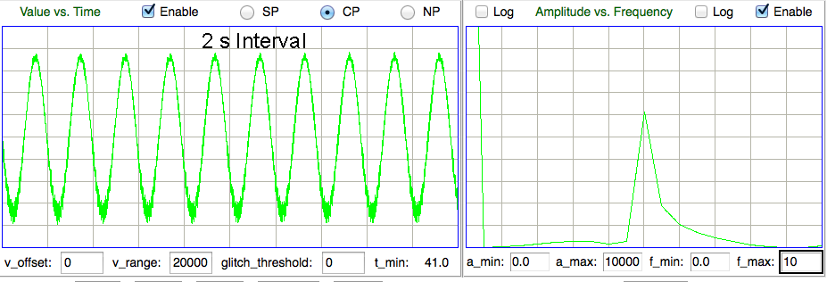
[25-MAY-17] A correspondant in the Netherlands uses TDT1 to translate a recording made with an ETA-F10 implantable monitor manufactured by DSI. His hope is to perform seizure detection with the Event Classifier. He applies a sinusoidal input to the device at frequencies 1 Hz, 5 Hz, 10 Hz, 20 Hz, 50 Hz, 100 Hz, 200 Hz, 500 Hz, 1000 Hz. The sample rate of the original signal is 1000 Hz, which we scale to 1024 Hz so we can apply a fast fourier transform to a one-second interval.
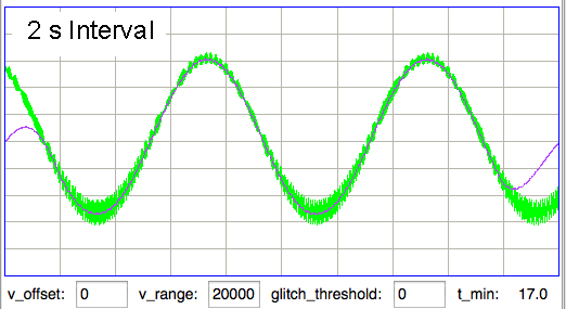
The spectrum of the 1-Hz fundamental is shown in here. Instead of a single peak at the fundamental frequency, we have a smeared peak after the fashion of a 1-Hz signal transmitted by frequency modulation. The ETA-F10 appears to emit pulses at a nominal frequency of 1 kHz, and modulates their frequency to indicate the signal voltage. The high-frequency artifact added to the sinusoid by the ETA-F10 has frequency 450-520 Hz. Because this artifact is greater on negative cycles of the sinusoide, it could easily be mistaken for a high frequency oscillation in the EEG. Knowing that this artifact exists, we can remove it with a 200-Hz low-pass filter. What remains below 200 Hz is a mild distortion of the 1-Hz waveform.
# Processor script to low-pass filter signal to 200 Hz.
Neuroplayer_band_power 0.1 200 1
scan [lwdaq ave_stdev $info(values)] %f%f%f%f%f ave stdev max min mad
append result "$info(channel_num) [format %.2f [expr 100.0 - $info(loss)]]\
	[format %.2f [expr 1.8*65536/$ave]] [format %.1f $stdev] "
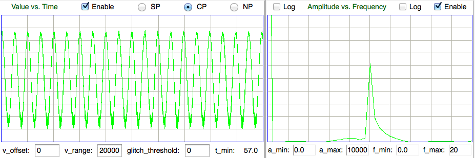
As we increase the frequency of the sinusoid, the amplitude of the signal drops as if there is a single-pole low-pass filter acting on the signal with corner frequency 100 Hz. At 200 Hz, we see distortion of the signal by a combination of modulation and aliasing, as is evident in the spectrum. The fundamental at 200 Hz is accompanied by another waveform at 290 Hz, and lower-frequency distortion at 50 Hz and 90 Hz.
Given that most interesting features in EEG are below 100 Hz, we recommend a pre-processing low-pass filter at 100 Hz for event detection in ETA-F10 recordings. A 100-Hz low-pass filter will remove most distortion of an EEG signal. When transients occur due to loss of signal or electrode movement, the high-frequency power in these steps will emerge from modulation and aliasing as low-frequency artifacts. A 100-Hz low-pass filter will not eliminate such artifacts.
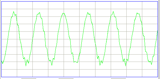
At the end of one of the recordings we have from an ETA-F10 transmitter made by DSI (see above), the animal dies. Following its death, we observe the following signal from the ETA-F10.

The above signal is the noise generated by an ETA-F10 while stationary in a conducting body. When the animal is alive, the baseline EEG amplitude is 25 μV rms.
[12-APR-10] We have five hours of data recorded at the Institute of Neurology (ION) at University College London (UCL) by Dr. Matthew Walker and his student Pishan Chang using the A3013A. The inverse-gain of this transmitter is 0.14 μV/count. Here we consider using the ratio of band powers to detect seizures. Using a power ratio has the potential advantage of making seizure detection independent of the sensitivity of individual implant electrodes.
When we tried to detect seizures by measuring power in the range 2-160 Hz, we found that step-like transient events also produced high power. We're not sure of the source of these transients, but we suspect they are the result of intermittent contact between two types of metal in the electrodes. We are sure they are not seizures. We define a seizure band, in which we expect epileptic seizures to exhibit most of their their power, and a transient band, in which we expect transient steps to exhibit power. In our initial experiments we choose 3-30 Hz for the seizure band and 0.2-2 Hz for the transient band. Seizures show up as power in the seizure band, but not in the transient band. Transients show up as power in both bands. When we see exceptional power in the seizure band, and the seizure power is five times greater than the transient power, we tag this interval as a candidate seizure. You can repeat our analysis with the following script.
set seizure_power [Neuroplayer_band_power 3 30 $config(enable_vt)]
set transient_power [Neuroplayer_band_power 0.2 2 0]
append result "$info(channel_num)\
  [format %.2f [expr 0.001 * $seizure_power]]\
  [format %.2f [expr 1.0 * $seizure_power / $transient_power]]"
if {($seizure_power > 1000000) \
  && ($seizure_power > [expr 5.0 * $transient_power])} {
  Neuroplayer_print "Seizure on $info(channel_num) at $config(play_time) s." purple
}
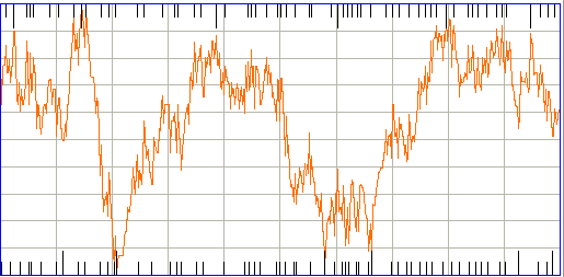
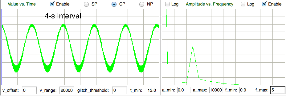
The following graphs show seizure-band power and seizure-transient power ratio for the first hour of our recording (M1262395837). We used window fraction 0.1 and glitch filter threshold 10,000 (1.4 mV). The playback interval was 4 s.
In these recordings, we convert band power to filtered signal amplitude with a = √(p/2) * 0.14 μV/count. Our seizure power threshold of 1 Msqcnt is the same as a seizure-band amplitude threshold of 100 μV. Our requirement that the seizure power be five times the transient power is the same as requiring that the seizure-band amplitude ba 2.2 times the transient-band amplitude.
Only the seizure activity confirmed by Dr. Walker on No1 has both high seizure power and high power ratio. There are sixteen 4-s intervals between 1244 s to 1336 s that qualify as seizures according to our criteria, and Dr. Walker agrees that they are indeed seizures. Channels No2 and No3 have many intervals with glitches and transients, but no seizures. Channel No7 has high power ratio in places, and at these times the signal looks like a seizure, but the power is below our threshold.
We apply the same processing to the remaining four hours of recordings. We see several more confirmed seizures on No1 up to a hundred seconds long. We see a few seizure-like intervals on No3 and No7. We cannot confirm whether these are short seizures or other activity. The following figure gives an example of such an interval.

Power ratios are useful in isolating seizures from the baseline signal, but we have been unable to isolate seizures using power ratios alone. In practice, we may have to rely upon consistency between implant electrodes so that we can use the amplitude of the signal as an additional isolation criterion.
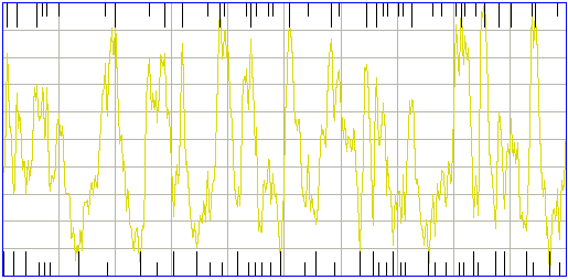
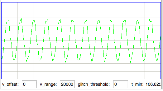
The EEG signals recorded at UCL from epileptic rats contain bursts of power in the range 60-100 Hz, with several bursts per second. The figure below gives an example.
The inverse-gain of the A3013A is 0.14 μV/count, so the burst has peak-to-peak amplitude of 500 μV. The following figure shows the same signal for a longer interval, showing how the bursts are repetitive.
We used the following processor script to detect wave bursts as well as seizures.
set seizure_power [expr 0.001 * [Neuroplayer_band_power 3 30 0]]
set burst_power [expr 0.001 * [Neuroplayer_band_power 40 160 $config(enable_vt)]]
set transient_power [expr 0.001 * [Neuroplayer_band_power 0.2 2 0]]
append result "$info(channel_num)\
  [format %.2f $transient_power]\
  [format %.2f $seizure_power]\
  [format %.2f $burst_power] "
if {($seizure_power > 1000) \
  && ($seizure_power > [expr 5.0 * $transient_power])} {
  Neuroplayer_print "Seizure on $info(channel_num) at $config(play_time) s." purple
}
if {($burst_power > 100) \
  && ($burst_power > [expr 0.5 * $transient_power])\
  && ($burst_power > $seizure_power)} {
  Neuroplayer_print "Wave burst on $info(channel_num) at $config(play_time) s." purple
}
The wave bursts on No3 in M1264098379 come and go for periods of a minute or longer. They are spread throughout the archive. When they occur, they often do so at roughly 5 Hz, but not always. In places, such as time 40 s, a single burst endures for a full second. The above script is effective at detecting all wave bursts, but it also responds to glitches too small for our glitch filter to eliminate. These glitches, caused by bad messages, were common before we introduced faraday enclosures and active antenna combiners to the recording system. Wave bursts are easy to detect using the 160-Hz bandwidth of the A3013A and A3019D.
[20-MAY-10] We receive from Sameer Dhamne (Children's Hospital Boston) a text file containing some EEG data they recorded from an epileptic rat. The header in the file says the sample rate is 400 Hz and the units of voltage are μV. There follows a list of 500k voltages, which covers a period of 1250 s. He asked us to import the data into the Neuroplayer and try our seizure-finding algorithm on it.
We remove the header from the file we received from Sameer and apply our translator. Our Fourier transform won't work on a number of samples that is not a perfect power of two, and our reconstruction won't work on a sample period that is not an integer multiple of the 32.768 kHz clock period. We don't need the reconstruction, since this data has no missing samples. So we turn it off. We use the Neuroplayer's Configuration Panel set the playback interval to a time that contains a number of samples that is an exact power of two. We now see the data and a spectrum.
[21-MAY-10] Our initial spectrum had a hole in it at 80 Hz, when we expect the hole to be at 60 Hz. We obtain the transform of the text file data using the following script, and plot the spectrum in Excel. We see a hole at 60 Hz.
set fn [LWDAQ_get_file_name]
set df [open $fn r]
set data [read $df]
close $df
set interval [lrange $data 0 4095]
set spectrum [lwdaq_fft $interval]
set f_step [expr 1.0*400/4096]
set frequency 0
foreach {a p} $spectrum {
  LWDAQ_print $t "[format %.3f $frequency] $a "
  set frequency [expr $frequency + $f_step]
}
We correct a bug in the translator, whereby we skip a sample whenever we insert a timestamp into the translated data, and our imported spectrum is now correct, as you can see below.

According to Sameer, the text data was recorded from a tethered rat. Here we see 5.12 s of the signal displayed, and its spectrum. There is a 60 Hz mains stop filter operating upon the signal. We see what appears to be an epileptic seizure taking place. This interval covers 1034 s to 1039 s from the start of the recording.
[06-AUG-10] At CHB, we have transmitter No.6 implanted, with electrodes cemented to the skull by silver epoxy. We record 1000 seconds in archive M1281121460. At time 936 s, we observe seizure-like activity, even though the rat is not epileptic. We observe the rat chewing the sanitary sheets shortly before and after we notice the signal.
We put the rat in a cage within the enclosure. It roams around. We record 140 seconds in archive M1281122799. We again notice seizure-like activity at various times, including 104 s. We apply our seizure-finding algorithm. It does not identify any seizures. We apply the script to an older archive M1262395837 from ION and detect this seizure during the 4-s interval after time 1248 s. The amplitude of the ION signal is greater and the frequency of the oscillations is higher than in the CHB signal. Peak power is at around 10 Hz in this seizure, while we see no definite peak power in the seizure-like signal.
[12-AUG-10] In archive M1281455686 recorded by Sameer Dhamne (Children's Hospital Boston), we see EEG from implanted transmitters No8 and No10. At time 1140 s, Sameer's iPhone interferes with radio-frequency reception. Reception from No8 drops to 0%. Reception from No10 drops to 70%. In a 4-s interval we receive 25 bad messages on channel No5. There are a similar number of bad messages in channel No10. The bad messages produce a seizure-like spectrum, as shown below.
We modify our seizure-detection so that it looks for seizures only when reception is robust (more than 80% of messages received).
[20-AUG-10] The TPSPBP processor calculates reception, transient power, seizure power, and burst power simultaneously for all selected channels. We apply the script to six hours of data starting with archive M1281985381 and ending with archive M1282081048. The following graph shows transient and seizure power during the 21,000 second period.
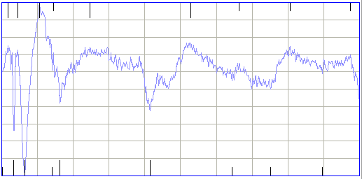
We see transient and seizure power jumping up for periods of a few minutes, growing more intense as time goes by. According to our earlier work, a seizure is characterized by high seizure power and low transient power, so we doubt that these events are seizures. The peak of seizure power corresponds to the following plot of EEG.
The plot shows oscillations at around 3 Hz, but also a swinging baseline, which gives rise to the transient power. We are not sure if this is a seizure or not. Other examples of the signal with high seizure power show larger swings in the baseline, 0.5-Hz pulses, and rapid, but not instant, changes in baseline potential.
[25-AUG-10] Receive another six hours of data from Sameer Dhamne (Children's Hospital Boston), starting with archive M1282668620 and ending with M1282686620. The rat was less active and more asleep during these six hours. We plot signal power here. There are no seizure-like events.
[04-APR-11] Joost Heeroma (Institute of Neurology, UCL) asks us to provide a scripts that will calculate the average power in various frequency bands over a period of an hour. We start with a script that calculates the power in several bands of interest. The Power Band Average (PBA.tcl) script for use with the Toolmaker. The script opens a file browser window and we select the characteristics files from which we want to calculate power averages. With the parameters given at the top of the script, we instruct the analysis on how many power bands are in each channel entry, which channels we want to analyze, and the length of the averaging period. The averages appear in the Toolmaker execution window. We cut and paste them into a spreadsheet, where we obtain plots of average power in all available bands.

We used the power average script to obtain the above graph of mains hum amplitude versus time as recorded by Louise Upton (Oxford University) in her office window over ninety hours. We see the power averaged over one-minute periods. A twenty-four hour cycle is evident, and some dramatic event in which the transmitter was moved upon its window sill.
[09-JUN-11] We have 67 hours of continuous recordings from two animals at CHB. Both animals have received an impact to their brains, and have developed epilepsy manifested in seizures of between one and four seconds duration. The transmitters are No4, and No5. The recordings cover 09-MAY-11 to 12-MAY-11 (archives M1304982132 to M1305220312). Our objective is to detect seizures with interval processing followed by interval analysis. The result will be a list of EEG events that we hope are seizures, giving the time of each seizure, its duration, some measure of its power, and an estimate of its spike frequency. The list should include at least 90% of the seizures that take place, and at the same time, 90% of the events in the list should be genuine seizures. We sent a list of 105 candidate seizures on No4 to Sameer. He and Alex looked through the list declared 83 of them to be seizures, while the remaining 22 were not. On the basis of these examples, we devised our ESP1 epileptic seizure processor and our SD3 seizure detection.
[19-JUN-11] We receive two text files from Sameer Dhamne (Children's Hospital Boston). They represent recordings made with tethered electrodes. Each line consists of a time, a comma, and a sample value. We assume the time is seconds from the beginning of the file and the sample is in microvolts. The samples occur every 2.5 ms for a sample frequency of 400 Hz. We give our text files names of the form Mxxxxxxxxxx.txt so that the TDT1 script will create archives of the form Mxxxxxxxxxx.ndf, which is what the Neuroplayer expects. We run the TDT1 script. We set the voltage range to ±13000 in the text file's voltage units. Because we assume the unit is μV, our range is therefore ±13 mV, which is the dynamic range of an A3019. We produce two archives, one 300 s and the other 600 s long. The script sets up the Neuroplayer to have default sample frequency 400 Hz and playback interval 1.28 s. These combine to create an interval with 512 samples, which is a perfect power of two, as required by our fast Fourier transform routine. We play back the archive and look for short seizures. Before we can return to play-back of A3019 archives, we must restore the default configuration of the Neuroplayer, such as sampling frequency of 512 SPS. The easiest way to do this is to close the Neuroplayer window and open it again.
[11-FEB-12] Our new TDT3 script allows us to extract up to fourteen signals from a text file database. The first line of the text file should give the names of the signals, and subsequent lines should give the signal values. There should be no time information in the first column. Instead, we tell the translator script the sample rate. We also tell it the full range of the signals for translation into our sixteen-bit format. We used this script to extract human EEG signals from text files we received from Athena Lemesiou (Institute of Neurology, UCL).
[27-APR-12] Our new TDT4 script allows us to extract all channels from a text file database and record them in multiple NDF files, with up to fourteen channels in each NDF file. The first line of the text file should give the names of the signals, and subsequent lines should give the signal values. The script records in the metadata of each NDF file the channel names and their corresponding NDF channel numbers within the NDF file. As in TDT3, we can set the full range of the signals for translation into our sixteen-bit format. Copy and paste the script into the LWDAQ Toolmaker and press Execute. The program is not fast: it takes two minutes on our laptop to translate ten minutes of data from sixty-four channels.
[10-OCT-12] We update our original TDT1 translator. The translator does not read the entire text file at the start, but goes through it line by line, thus allowing it to deal with arbitrarily large files. It writes the channel names and numbers to the metadata of the translated archive.
[10-APR-13] We improve TDT1 so that it records more details of the translation in the ndf metadata. We fix problems in the Neuroplayer that stopped it working with translated archives of sample rate 400 SPS.
[11-MAY-25] See our Example Recordings page for packages of telemetry recordings, characteristics files, event classification processors, batch processing scripts that operate together to demonstrate automatic event classification. In the paragraphs below we provide brief examples of classification in the field.
[12-MAY-25] We have twenty-four hours of test EEG data from nine A3049H2 transmitters and Kings College London (KCL). These are two-channel 0.2-80 Hz devices implanted to record two channels of EEG each. We also have five hours recorded on a different day from which we are to develop our ictal event library. We have a list of ictal events made for us by KCL, which we use as the basis for a new and smaller event library. We are looking for short seizures lasting one or two seconds. Our objective is to count the hourly number of seconds that contain ictal spikes. We play through the library archives with a one-second interval and build Lib12MAY25KH consisting of 37 in total, a third baseline, third ictal. We use the ECP20V3 processor, which is optimized for 80-Hz bandwidth. We find that the coherence metric does most of the work of distinguishing the ictal intervals, and coastline gives the greatest separation of baseline and ictal.
We apply ECP20V3 the twenty-four hours of test recording, processing one-second intervals and writing to disk for all channels. This takes our laptop several hours. We use our library to perform batch classification using coastline and coherence with match limit 0.05 and power threshold 0.0. These are two-channel transmitters, and in our experience, ictal events usually show up in both channels within a few seconds, so we expect the number of ictal events in the two channels of each transmitter to be similar. We provide the Batch Classifier summary output below. It's a little hard to decypher without color coding, but we have channel number and ictal interval count for each channel in each hour.
M1734130922_ECP20V3R1.txt 1 0 2 2 5 62 6 83 7 75 8 120 9 5 10 24 13 1 14 6 17 0 18 17 21 0 22 1 23 0 24 3 25 77 26 97
M1734134523_ECP20V3R1.txt 1 20 2 48 5 9 6 9 7 90 8 142 9 0 10 0 13 0 14 1 17 1 18 19 21 35 22 66 23 0 24 23 25 43 26 43
M1734138124_ECP20V3R1.txt 1 3 2 3 5 66 6 78 7 64 8 129 9 0 10 0 13 70 14 71 17 103 18 204 21 0 22 0 23 0 24 0 25 0 26 0
M1734141725_ECP20V3R1.txt 1 0 2 0 5 174 6 151 7 317 8 479 9 21 10 125 13 189 14 129 17 257 18 383 21 0 22 1 23 0 24 1 25 0 26 0
M1734145326_ECP20V3R1.txt 1 0 2 0 5 0 6 0 7 228 8 352 9 30 10 101 13 106 14 85 17 163 18 316 21 0 22 1 23 0 24 0 25 0 26 0
M1734148927_ECP20V3R1.txt 1 0 2 0 5 213 6 166 7 173 8 310 9 0 10 0 13 95 14 78 17 150 18 253 21 138 22 128 23 0 24 0 25 0 26 0
M1734152528_ECP20V3R1.txt 1 29 2 51 5 119 6 74 7 74 8 155 9 0 10 1 13 0 14 4 17 48 18 171 21 28 22 46 23 0 24 0 25 0 26 0
M1734156129_ECP20V3R1.txt 1 2 2 25 5 0 6 3 7 1 8 3 9 0 10 0 13 0 14 2 17 2 18 10 21 20 22 32 23 1 24 22 25 0 26 1
M1734159730_ECP20V3R1.txt 1 33 2 47 5 149 6 106 7 159 8 312 9 31 10 219 13 14 14 28 17 18 18 48 21 107 22 76 23 8 24 49 25 51 26 153
M1734163331_ECP20V3R1.txt 1 28 2 35 5 154 6 107 7 288 8 420 9 17 10 102 13 141 14 101 17 119 18 214 21 19 22 30 23 2 24 40 25 46 26 165
M1734166932_ECP20V3R1.txt 1 21 2 56 5 190 6 121 7 335 8 491 9 5 10 28 13 94 14 104 17 152 18 259 21 157 22 143 23 8 24 93 25 155 26 225
M1734170533_ECP20V3R1.txt 1 24 2 60 5 108 6 66 7 196 8 364 9 20 10 173 13 194 14 140 17 197 18 328 21 170 22 160 23 11 24 132 25 154 26 188
M1734174134_ECP20V3R1.txt 1 26 2 39 5 170 6 89 7 206 8 294 9 13 10 86 13 45 14 42 17 110 18 269 21 130 22 124 23 15 24 68 25 97 26 151
M1734177735_ECP20V3R1.txt 1 3 2 14 5 253 6 163 7 150 8 288 9 16 10 137 13 90 14 84 17 137 18 234 21 184 22 157 23 4 24 90 25 158 26 204
M1734181336_ECP20V3R1.txt 1 24 2 33 5 243 6 134 7 310 8 416 9 13 10 73 13 79 14 72 17 166 18 323 21 77 22 95 23 15 24 85 25 77 26 115
M1734184937_ECP20V3R1.txt 1 31 2 45 5 122 6 94 7 305 8 484 9 8 10 58 13 50 14 60 17 94 18 166 21 92 22 113 23 1 24 30 25 25 26 64
M1734188538_ECP20V3R1.txt 1 15 2 23 5 271 6 174 7 309 8 416 9 15 10 107 13 128 14 110 17 206 18 384 21 109 22 99 23 10 24 91 25 47 26 63
M1734192139_ECP20V3R1.txt 1 46 2 62 5 40 6 22 7 79 8 174 9 11 10 105 13 49 14 66 17 97 18 190 21 86 22 105 23 5 24 61 25 104 26 144
M1734195740_ECP20V3R1.txt 1 25 2 37 5 202 6 145 7 232 8 359 9 9 10 72 13 120 14 91 17 186 18 317 21 198 22 116 23 6 24 78 25 58 26 91
M1734199341_ECP20V3R1.txt 1 36 2 52 5 62 6 36 7 196 8 277 9 16 10 65 13 75 14 71 17 149 18 258 21 129 22 104 23 16 24 81 25 76 26 66
M1734202942_ECP20V3R1.txt 1 12 2 1 5 11 6 7 7 8 8 15 9 4 10 40 13 1 14 2 17 21 18 45 21 6 22 2 23 0 24 9 25 21 26 34
M1734206543_ECP20V3R1.txt 1 2 2 0 5 67 6 57 7 142 8 228 9 0 10 0 13 9 14 9 17 14 18 38 21 1 22 1 23 2 24 20 25 137 26 86
M1734210144_ECP20V3R1.txt 1 31 2 44 5 33 6 62 7 153 8 230 9 0 10 0 13 89 14 81 17 48 18 114 21 78 22 71 23 4 24 62 25 39 26 37
M1734213745_ECP20V3R1.txt 1 7 2 4 5 22 6 30 7 81 8 164 9 37 10 100 13 4 14 12 17 8 18 19 21 0 22 1 23 0 24 2 25 109 26 118
Total of 1555200 intervals, 60873 with signal loss, 1494327 above threshold, 36716 matched types.
We see order of magnitude agreement in the number of ictal intervals between most pairs of channels. Channels No23 and No24 are an exception, we see No24 with almost ten times as many ictal intervals. In total, we have a total of 37k ictal events our of 1.6M intervals. Our Ictal rate is 2.3%. We load the ictal event list into the Neuroplayer with the Load button in the Events line. We use the Hop button to hop around in the event list at random. Out of 109 events, we judge by eye that 100 are ictal and 9 are baseline. All 9 that we deem to be baseline are still borderline ictal. Of our ictal intervals, 8.2% are false positives. Our total false positive rate is 0.2%, which is ten times less than our true event rate. We play through several archives and see no instances of an ictal event being missed, so our false negative rate must be less than 10%. We zip up the recordings, the processor, the library, the characteristics, and the final event list into ECP20_12MAY25.zip (Warning: 1500 MByte download).
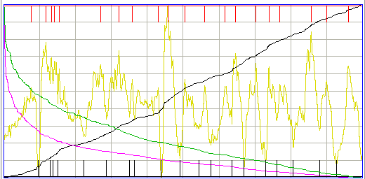
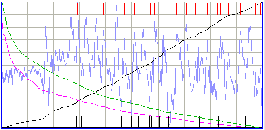
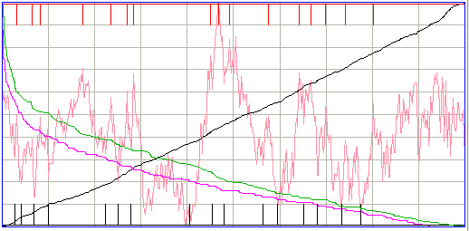
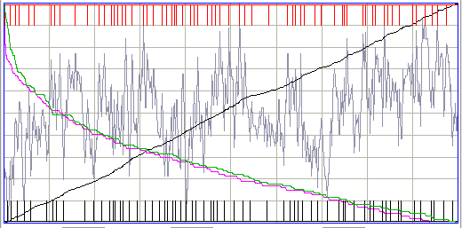
[13-MAY-25] On the advice of a colleague, we make the following histograms of the six metrics over our 1.5 million channel-seconds of characterized recordings using Toolmaker script Metric_Histogram.tcl.

The sharp aberrations we suspect are an artifact of our histogram calculation: a rounding error of some kind. We will look into the cause. Our ictal event detector is driven primarily by the coherence metric. The histogram of coherence shows no bump at high coherence corresponding to ictal events. Our ictal event detection is approximately a cut we make in the histogram of coherence at about 0.7. Anything with coherence above 0.7, provided it has coastling 0.30-0.57, we classify as ictal.